Kaggle信用卡欺诈数据

参考链接
https://www.cnblogs.com/bonelee/p/9087882.html
https://blog.csdn.net/nlpuser/article/details/81265614
https://www.cnblogs.com/gczr/p/6802948.html

数据预处理

import pandas as pd
data=pd.read_csv(r'D:\dataanalysis\creditcard.csv',sep=',')#导入数据
data.info()#查看数据字段
data.shape#查看数据大小

data[data.isnull().values==True] #缺失值查找 
data['Hour']=data["Time"].apply(lambda x : divmod(x, 3600)[0])#把时间转化为小时为单位

#对Amount和Hour进行标准化
from sklearn.preprocessing import StandardScaler # 导入模块
sc =StandardScaler() # 初始化缩放器
data[['Amount','Hour']] =sc.fit_transform(data[['Amount','Hour']])#对数据进行标准化

data_fruad=data[data['Class']==1]#欺诈数据
data_notfruad=data[data['Class']==0]#非欺诈数据

箱线图

#画出欺诈数据各指标的箱线图
import matplotlib.pyplot as plt
plt.rcParams['font.sans-serif'] = ['SimHei'] #用来正常显示中文标签
plt.rcParams['axes.unicode_minus'] = False #用来正常显示负号
plt.figure(figsize=(15,6))
data_fruad[['V1','V2','V3','V4','V5','V6','V7','V8','V9','V10','V11','V12','V13','V14','V15','V16','V17','V18','V19','V20','V21','V22','V23','V24','V25','V26','V27','V28','Amount','Hour']].boxplot()
plt.title('欺诈数据各指标箱线图',fontsize=20)
plt.xlabel('各项指标',fontsize=18)
plt.ylabel('各项指标大小',fontsize=18)
plt.xticks(rotation=90)#旋转横坐标
plt.tick_params(labelsize=16)#增大横坐标刻度大小
plt.show()

#要画非欺诈样本和总样本的各指标箱线图只需将data_fruad换成data_nonfruad/data

箱线图如下



可以看出欺诈样本和非欺诈样本之间的分布是有很大区别的，由于非欺诈样本每个变量的范围较大，看不清箱线图的箱体，把非欺诈样本的箱线图纵向拉长，如下：

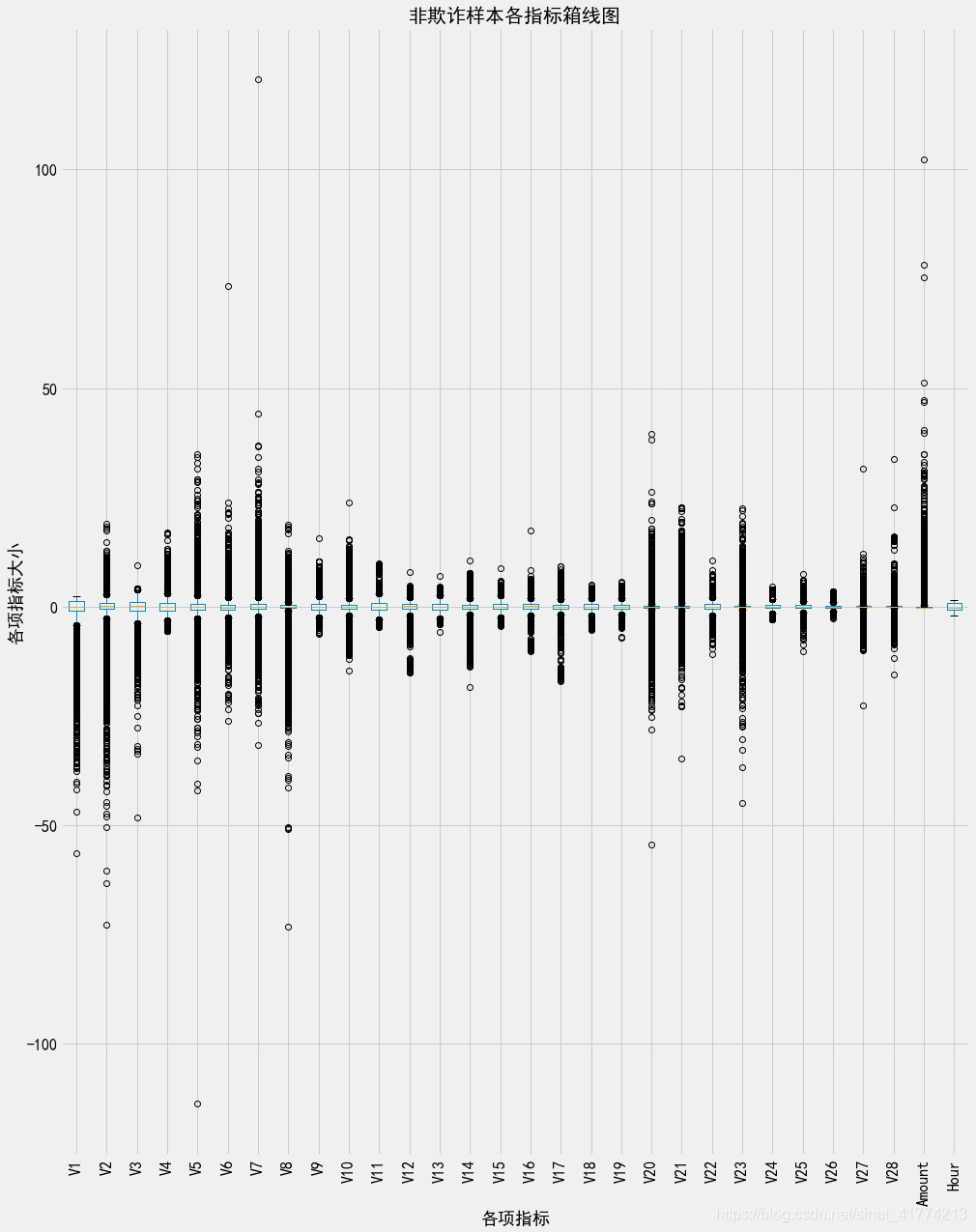
可以看出，正常样本的每个指标变量的箱体都是在0上，即正常样本的分布都是关于0对称的，而欺诈样本的箱体明显在0的左右波动，呈现明显的左偏或右偏。

热力图

#画变量之间相关性的热力图
import seaborn as sns
x_feature = list(data.columns)
x_feature.remove('Time')
x_feature.remove('Class')
corr_fruad=data_fruad[x_feature].corr()
corr_fruad=abs(corr_fruad)
corr_notfruad=data_notfruad[x_feature].corr()
corr_notfruad=abs(corr_notfruad)
f,(ax1,ax2)=plt.subplots(figsize=(14,10),nrows=2)
#cmap = sns.cubehelix_palette(start = 1.5, rot = 3, gamma=0.8, as_cmap = True)
sns.heatmap(corr_fruad,ax=ax1,vmax=1,vmin=0,annot=False,linewidths=0.05,cmap='rainbow')
ax1.set_title('fruad data heatmap')
ax1.set_xlabel('variables')
ax1.set_xticklabels([]) #设置x轴图例为空值
ax1.set_ylabel('variables')
sns.heatmap(corr_notfruad,ax=ax2,vmax=1,vmin=0,annot=False,linewidths=0.05,cmap='rainbow')
ax2.set_title('nonfruad data heatmap')
ax2.set_xlabel('variables')
ax2.set_ylabel('variables')
plt.show()

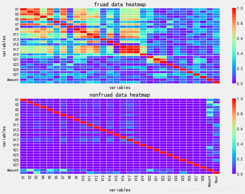
欺诈样本中V19之前的大部分指标之间有明显的相关性

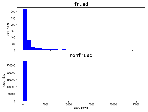
Amount直方图

#Amount的直方图
f,(ax1,ax2)=plt.subplots(figsize=(8,6),nrows=2)
ax1.hist(data_fruad['Amount'],bins=30,color='b')
ax1.set_ylabel('counts',fontsize=15)
ax1.set_xticklabels([]) 
ax1.set_title('fruad',fontsize=20)

ax2.hist(data_notfruad['Amount'],bins=30,color='b')
ax2.set_ylabel('counts',fontsize=15)
ax2.set_xlabel('Amounts',fontsize=15)
ax2.set_title('nonfruad',fontsize=20)

特征选择

1、根据每个变量的欺诈样本和正常样本的分布的差异情况，如果欺诈样本和正常样本的分布差异不大，则可以去除该特征。

from matplotlib import gridspec
plt.figure(figsize=(16,30*4))
gs = gridspec.GridSpec(30, 1)#创建20行1列的画布
for i, cn in enumerate(data[x_feature]):
    ax = plt.subplot(gs[i])
    sns.distplot(data[cn][data["Class"] == 1], bins=50)
    sns.distplot(data[cn][data["Class"] == 0], bins=100)
    ax.set_xlabel('')
    ax.set_title('histogram of feature: ' + str(cn))

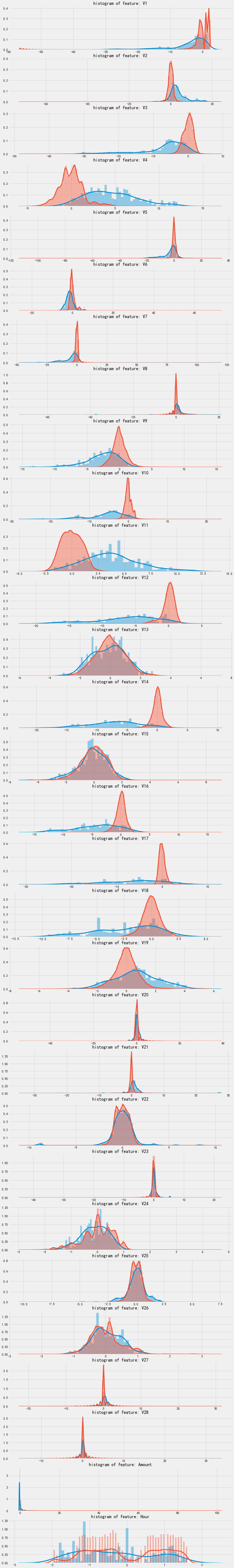
可以剔除变量V8 V13 V16 V20 V22 V23 V25 V26 V27 V28

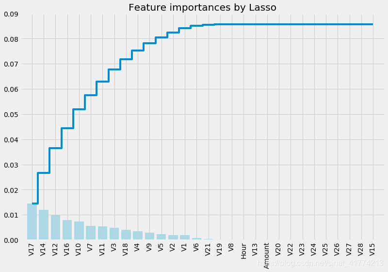
2、用Lasso进行变量选择

#进行变量选择
from sklearn.linear_model import Ridge, RidgeCV, ElasticNet, LassoCV, LassoLarsCV
from sklearn.model_selection import cross_val_score

x_values=data[x_feature]
y_values=data['Class']

#调用LassoCV函数，并进行交叉验证，默认cv=3
model_lasso = LassoCV(alphas = [0.1,1,0.001, 0.0005]).fit(x_values, y_values)

#输出看模型最终选择了几个特征向量，剔除了几个特征向量
coef = pd.Series(model_lasso.coef_, index = x_feature)
print("Lasso picked " + str(sum(coef != 0)) + " variables and eliminated the other " +  str(sum(coef == 0)) + " variables")

#可视化各变量的重要程度
import numpy as np
import matplotlib.pyplot as plt
plt.style.use('fivethirtyeight')  #其中的一种主题，可以通过plt.style.availabel查看有多少种主题
names = data[x_feature].columns
importances = np.abs(model_lasso.coef_)
feat_names = names
indices = np.argsort(importances)[::-1]  #按照重要顺序从小到大排序并获取逆序索引
fig = plt.figure(figsize=(12,8))
plt.title("Feature importances by Lasso")
plt.bar(range(len(indices)), importances[indices], color='lightblue',  align="center")
plt.step(range(len(indices)), np.cumsum(importances[indices]), where='mid', label='Cumulative')
plt.xticks(range(len(indices)), feat_names[indices], rotation='vertical',fontsize=14)
plt.xlim([-1, len(indices)])
plt.show()

3、随机森林分类器对特征重要性进行排序

#利用随机森林的feature importance对特征的重要性进行排序
from sklearn.ensemble import RandomForestClassifier
names = data[x_feature].columns
clf=RandomForestClassifier(n_estimators=10,random_state=123)#构建分类随机森林分类器
clf.fit(x_values, y_values) #对自变量和因变量进行拟合
for feature in zip(names, clf.feature_importances_):
    print(feature)

#可视化由随机森林分类器判定的各类的重要顺序
import numpy as np
import matplotlib.pyplot as plt
plt.style.use('fivethirtyeight')#其中的一种主题，可以通过plt.style.availabel查看有多少种主题
#plt.rcParams['figure.figsize'] = (12,6)#设置画布尺寸
importances = clf.feature_importances_
feat_names = names
indices = np.argsort(importances)[::-1]#按照重要顺序从小到大排序并获取逆序索引
fig = plt.figure(figsize=(12,6))
plt.title("Feature importances by RandomTreeClassifier")
plt.bar(range(len(indices)), importances[indices], color='lightblue',  align="center")
plt.step(range(len(indices)), np.cumsum(importances[indices]), where='mid', label='Cumulative')
plt.xticks(range(len(indices)), feat_names[indices], rotation='vertical',fontsize=14)
plt.xlim([-1, len(indices)])
plt.show()

处理样本不平衡问题（SMOTE模块）

#处理样本的不平衡问题
from imblearn.over_sampling import SMOTE # 导入SMOTE算法模块
sm = SMOTE(random_state=42)    # 处理过采样的方法
X=data[x_feature]
y=data['Class']
X, y = sm.fit_sample(X, y)

n_sample = y.shape[0]
n_pos_sample = y[y == 0].shape[0]
n_neg_sample = y[y == 1].shape[0]
print('通过SMOTE方法平衡正负样本后')
print('样本个数：{}; 正样本占{:.2%}; 负样本占{:.2%}'.format(n_sample,n_pos_sample/n_sample,n_neg_sample/n_sample))

LogisticRegression（使用的原始特征）

#划分训练集和测试集
from sklearn.model_selection import train_test_split
X_train, X_test, y_train, y_test = train_test_split(X, y, test_size = 0.3, random_state = 0) # test_size是样本占比，random_state是随机数种子编号，0表示每次切分的数据都一样

from sklearn.metrics import accuracy_score
from sklearn.model_selection import GridSearchCV
from sklearn.linear_model import LogisticRegression
from sklearn.metrics import classification_report

# 构建参数组合，其中penalty表示惩罚项
param_grid = {'C': [0.01,0.1, 1, 10, 100, 1000,],'penalty': [ 'l1', 'l2']}

#GridSearchCV用于系统地遍历多种参数组合，通过交叉验证确定最佳效果参数
#确定模型LogisticRegression，和参数组合param_grid ，cv指定10折
grid_search=GridSearchCV(LogisticRegression(),param_grid,cv=10) 

grid_search.fit(X_train, y_train) # 使用训练集学习算法

y_pred = grid_search.predict(X_test)#测试集预测值
print("Test set accuracy score: {:.5f}".format(accuracy_score(y_test, y_pred,)))#测试集预测精度
print(classification_report(y_test, y_pred))

Test set accuracy score: 0.94805

          precision    recall  f1-score   support
 0         0.92      0.98      0.95     85172
 1         0.97      0.92      0.95     85417

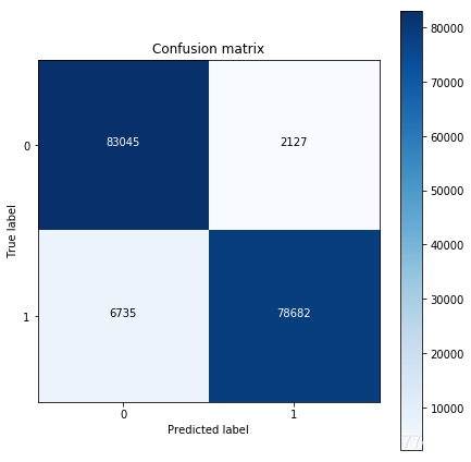
#混淆矩阵可视化
from sklearn.metrics import confusion_matrix
import numpy as np
import matplotlib.pyplot as plt

cnf_matrix = confusion_matrix(y_test, y_pred)  # 生成混淆矩阵
np.set_printoptions(precision=2)
print("Recall metric in the testing dataset: ", cnf_matrix[1,1]/(cnf_matrix[1,0]+cnf_matrix[1,1]))

import itertools
def plot_confusion_matrix(cm, classes,title='Confusion matrix',cmap=plt.cm.Blues):
    """
    This function prints and plots the confusion matrix.
    """
    plt.imshow(cm, interpolation='nearest', cmap=cmap)
    plt.title(title)
    plt.colorbar()
    tick_marks = np.arange(len(classes))
    plt.xticks(tick_marks, classes, rotation=0)
    plt.yticks(tick_marks, classes)

    thresh = cm.max() / 2.
    for i, j in itertools.product(range(cm.shape[0]), range(cm.shape[1])):
        plt.text(j, i, cm[i, j],
                 horizontalalignment="center",
                 color="white" if cm[i, j] > thresh else "black")

    plt.tight_layout()
    plt.ylabel('True label')
    plt.xlabel('Predicted label')

class_names = [0,1]
plt.figure(figsize=(6,6))
plot_confusion_matrix(cnf_matrix,classes=class_names,title='Confusion matrix')
plt.show()

Recall metric in the testing dataset: 0.9211515272135523

y_pred_proba = grid_search.predict_proba(X_test)  #predict_prob 获得一个概率值
thresholds = [0.1,0.2,0.3,0.4,0.5,0.6,0.7,0.8,0.9]  # 设定不同阈值
plt.figure(figsize=(15,10))
j = 1
for i in thresholds:
    y_test_predictions_high_recall = y_pred_proba[:,1] > i#预测出来的概率值是否大于阈值 
    plt.subplot(3,3,j)
    j += 1
    # Compute confusion matrix
    cnf_matrix = confusion_matrix(y_test, y_test_predictions_high_recall)
    np.set_printoptions(precision=2)
    print("Recall metric in the testing dataset: ", cnf_matrix[1,1]/(cnf_matrix[1,0]+cnf_matrix[1,1]))
    # Plot non-normalized confusion matrix
    class_names = [0,1]
    plot_confusion_matrix(cnf_matrix,classes=class_names)
plt.show()

Recall metric in the testing dataset: 0.986162005221443
Recall metric in the testing dataset: 0.9673250055609539
Recall metric in the testing dataset: 0.9485348349860098
Recall metric in the testing dataset: 0.9346968402074528
Recall metric in the testing dataset: 0.9211515272135523
Recall metric in the testing dataset: 0.9085545032019388
Recall metric in the testing dataset: 0.8970813772434059
Recall metric in the testing dataset: 0.886287273025276
Recall metric in the testing dataset: 0.8708453820668017

from itertools import cycle
from sklearn.metrics import precision_recall_curve
from sklearn.metrics import auc
from sklearn.metrics import roc_auc_score
from sklearn.metrics import roc_curve
from sklearn.metrics import recall_score

thresholds = [0.1,0.2,0.3,0.4,0.5,0.6,0.7,0.8,0.9]
colors = cycle(['navy', 'turquoise', 'darkorange', 'cornflowerblue', 'teal', 'red', 'yellow', 'green', 'blue','black'])

plt.figure(figsize=(12,7))

j = 1
for i,color in zip(thresholds,colors):
    y_test_predictions_prob = y_pred_proba[:,1] > i #预测出来的概率值是否大于阈值  

    precision, recall, thresholds = precision_recall_curve(y_test, y_test_predictions_prob)
    area = auc(recall, precision)
    
    # Plot Precision-Recall curve
    plt.plot(recall, precision, color=color,
                 label='Threshold: %s, AUC=%0.5f' %(i , area))
    plt.xlabel('Recall')
    plt.ylabel('Precision')
    plt.ylim([0.0, 1.05])
    plt.xlim([0.0, 1.0])
    plt.title('Precision-Recall Curve')
    plt.legend(loc="lower left")
plt.show()

随机森林分类器（使用的原始特征）

#过抽样
sm = SMOTE(random_state=42)    # 处理过采样的方法
X=data[x_feature]
y=data['Class']
X,y= sm.fit_sample(X,y)

#划分训练集
X_RFtrain, X_RFtest, y_RFtrain, y_RFtest = train_test_split(X, y, test_size = 0.3, random_state = 0)

#利用随机森林分类器
from sklearn.ensemble import RandomForestClassifier
from sklearn.model_selection import cross_val_score
clf_RF=RandomForestClassifier(n_estimators=10,random_state=123)#构建分类随机森林分类器
clf_RF.fit(X_RFtrain,y_RFtrain)

#交叉验证
scores_RF=cross_val_score(clf_RF,X_RFtrain,y_RFtrain)
print('RandomForestClassifier交叉验证准确率为:'+str(scores_RF.mean()))

RandomForestClassifier交叉验证准确率为:0.9998090649079457

y_RFpred= clf_RF.predict(X_RFtest)#进行预测
print("Test set accuracy score: {:.5f}".format(accuracy_score(y_test, y_pred,)))#测试集预测精度
print(classification_report(y_RFtest,y_RFpred))

Test set accuracy score: 0.93732

             precision    recall  f1-score   support
       0       1.00      1.00      1.00     85172
       1       1.00      1.00      1.00     85417

# 生成混淆矩阵
cnf_matrix_RF= confusion_matrix(y_RFtest,y_RFpred)  
np.set_printoptions(precision=2)
print("Recall metric in the testing dataset: ", cnf_matrix_RF[1,1]/(cnf_matrix_RF[1,0]+cnf_matrix_RF[1,1]))

#画混淆矩阵
class_names = [0,1]
plt.figure(figsize=(6,6))
plot_confusion_matrix(cnf_matrix_RF,classes=class_names,title='Confusion matrix')
plt.show()

Recall metric in the testing dataset: 0.9999882927286138

随机森林分类效果超好

LogisticRegression（使用LASSO特征选择后的特征）

#lasso删去'V8','V13','V15','V20','V22','V23','V24','V25','V26','V27','V28','Amount','Hour'
x_feature.remove('V8')
x_feature.remove('V13')
x_feature.remove('V15')
x_feature.remove('V20')
x_feature.remove('V22')
x_feature.remove('V23')
x_feature.remove('V24')
x_feature.remove('V25')
x_feature.remove('V26')
x_feature.remove('V27')
x_feature.remove('V28')
x_feature.remove('Amount')
x_feature.remove('Hour')

sm = SMOTE(random_state=42)    # 处理过采样的方法
X=data[x_feature]
y=data['Class']
X, y = sm.fit_sample(X, y)
X_train, X_test, y_train, y_test = train_test_split(X, y, test_size = 0.3, random_state = 0)#划分训练集

# 构建参数组合，其中penalty表示惩罚项
param_grid = {'C': [0.01,0.1, 1, 10, 100, 1000,],'penalty': [ 'l1', 'l2']}
#GridSearchCV用于系统地遍历多种参数组合，通过交叉验证确定最佳效果参数
grid_search=GridSearchCV(LogisticRegression(),param_grid,cv=10) 
grid_search.fit(X_train, y_train) # 使用训练集学习算法
y_pred = grid_search.predict(X_test)#测试集预测值
print("Test set accuracy score: {:.5f}".format(accuracy_score(y_test, y_pred,)))#测试集预测精度
print(classification_report(y_test, y_pred))

Test set accuracy score: 0.93732

              precision    recall  f1-score   support
       0       0.91      0.97      0.94     85172
       1       0.97      0.90      0.94     85417

而使用原始变量进行LR分类时测试集结果如下：
Test set accuracy score: 0.94805

          precision    recall  f1-score   support
 0         0.92      0.98      0.95     85172
 1         0.97      0.92      0.95     85417

进行变量选择之后的效果没有原始的效果好了