"""
    信用卡欺诈检测
    时间:2018\9\24 0024
"""
import time
import pandas as pd
import matplotlib.pyplot as plt
import numpy as np

"""
    读取csv文件:
"""
# pandas读取此数据巨慢,测试用时167s,分段读取拼接后,测试用时不到20s


init_time = time.time()
loop = True
f = open('creditcard.csv')
data = pd.read_csv(f, iterator = True)
chunkSize = 5000
chunks = []
while loop:
    try:
        chunk = data.get_chunk(chunkSize)
        chunks.append(chunk)
    except StopIteration:
        loop = False
        print("Iteration is stopped")
data = pd.concat(chunks, ignore_index = True)  # 拼接分段读取的数据。
print(data.head(), "\n", data.shape, "\n", type(data))
print(time.time() - init_time)
运行结果:
D:\Python\python.exe G:/编程/python/project/TYD/01/01/10/creditcard.py
Iteration is stopped
Time V1 V2 V3 ... V27 V28 Amount Class
0 0.0 -1.359807 -0.072781 2.536347 ... 0.133558 -0.021053 149.62 0
1 0.0 1.191857 0.266151 0.166480 ... -0.008983 0.014724 2.69 0
2 1.0 -1.358354 -1.340163 1.773209 ... -0.055353 -0.059752 378.66 0
3 1.0 -0.966272 -0.185226 1.792993 ... 0.062723 0.061458 123.50 0
4 2.0 -1.158233 0.877737 1.548718 ... 0.219422 0.215153 69.99 0
[5 rows x 31 columns]
(284807, 31)
<class 'pandas.core.frame.DataFrame'>
15.871907949447632
Process finished with exit code 0
"""
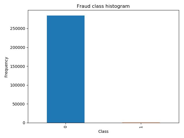
0属于正常的,占绝大部分
1属于异常的,占很小的部分
数据中,Class相当于Y;前边的数据,相当于X。
"""
count_classes = pd.value_counts(data['Class'], sort = True).sort_index() # value_counts计算Class里有多少个属性值
count_classes.plot(kind = 'bar') # 用图表表示出来
plt.title('Fraud class histogram')
plt.xlabel('Class')
plt.ylabel('Frequency')
plt.show()
运行结果:
说明:
可以看出0样本奖金有28万个,1样本基本很少。
样本极度不均衡
2种解决方案:
1,过采样:
在1号样本里生成出来的一些数据,生成出的数据跟0号样本一样多,也就是1号样本生成20多万条数据。
2,下采样:
两个数据样本不均衡,可以让0和1一样少就行了,多的里边选出来跟少的一样多,再把选出来的0和1组合在一起。
过采样对应的同样多,下采样对应的同样少
再做数据均衡之前,需要做另外一件事:
Amount列,数据差异比较大机器学习算法认为数值偏大的数据权重较高,数值较小的数据权重较低,为了使得每一个特征权重相当,需要将数据标准化
"""
    利用sklearn库标准化数据
"""
data['normAmount'] = StandardScaler().fit_transform(data['Amount'].values.reshape(-1, 1))
data = data.drop(['Time', 'Amount'], axis = 1)  # 丢弃Time列,Amount列
print(data.head())
# data['normAmount']表示添加一列,fit_transform填充并转换,reshape(-1是自动识别行数, 1列数)
# pandas的Series对象没有reshape方法,用values方法将Series对象转化成numpy的ndarray,再用ndarray的reshape方法
运行结果:
V1 V2 V3 ... V28 Class normAmount
0 -1.359807 -0.072781 2.536347 ... -0.021053 0 0.244964
1 1.191857 0.266151 0.166480 ... 0.014724 0 -0.342475
2 -1.358354 -1.340163 1.773209 ... -0.059752 0 1.160686
3 -0.966272 -0.185226 1.792993 ... 0.061458 0 0.140534
4 -1.158233 0.877737 1.548718 ... 0.215153 0 -0.073403
[5 rows x 30 columns]
Process finished with exit code 0
"""
    下采样
"""
# 取特征数据
X = data.loc[:, data.columns != 'Class']  # 取data中的不包含Class列,iloc根据行标签获取数据
Y = data.loc[:, data.columns == 'Class']  # 取data中的Class列
# 计算Class为1的样本都多少个:
number_records_fraud = len(data[data.Class == 1])  # 样本个1的个数
fraud_indices = np.array(data[data.Class == 1].index)  # 样本1的index值
# 取出Class为0的样本的index,因为是下采样,则0样本需要往少的取:
normal_indices = data[data.Class == 0].index
# 随机选择样本0,
# choice(什么样的地方随机选择,随机选择个数)返回index值
random_normal_indices = np.random.choice(normal_indices, number_records_fraud, replace = False)
random_normal_indices = np.array(random_normal_indices)
# 合并两种index的样本的index
under_sample_indices = np.concatenate([fraud_indices, random_normal_indices])  # 样本1,随机的样本0
# 取出两种样本的实际数据
under_sample_data = data.iloc[under_sample_indices, :]  # iloc根据行号获取数据
# 分成X和Y
# 此处原来是ix,现在pandas已弃用ix,ix表示可以根据行标签或者行号获取数据,容易造成混淆
X_undersample = under_sample_data.loc[:, under_sample_data.columns != 'Class']
Y_undersample = under_sample_data.loc[:, under_sample_data.columns == 'Class']
# 打印出数据个数和占比
print('Fraud:', len(under_sample_data[under_sample_data.Class == 1]) / len(under_sample_data))
print('Normal', len(under_sample_data[under_sample_data.Class != 1]) / len(under_sample_data))
print('All:', len(under_sample_data))
运行结果:
Fraud: 0.5
Normal 0.5
All: 984
交叉验证:
通常将一整份数据集按照28开,其中80%用来做训练集,20%用来做测试集

参数训练完成之后,为了模型参数的稳定性,
我们将训练集再平均分成3份,用来互相验证


其中用来验证的③,②,①我们成为验证集,可以看出,验证集包含在训练集的内部,并且是随机的切分操作。
"""
    交叉验证
"""
"""
    新的模块sklearn.model_selection,
    将以前的
    sklearn.cross_validation,
    sklearn.grid_search和
    sklearn.learning_curve模块组合到一起
"""

from sklearn.model_selection import train_test_split

# (X,Y,切分比例,随机状态0为最大程度随机)
# 此处的X,Y指的是全部数据集中的X和Y
X_train, X_test, Y_train, Y_test = train_test_split(X, Y, test_size = 0.3, random_state = 0)
print('X_train length:', len(X_train))
print('X_test length:', len(X_test))
print('X_test+X_train length:', len(X_train) + len(X_test))

# 此处的X,Y指的是下采样之后的的X和Y
X_train_undersample, X_test_undersample, Y_train_undersample, Y_test_undersample = train_test_split(X_undersample,
                                                                                                    Y_undersample,
                                                                                                    test_size = 0.3,
                                                                                                    random_state = 0)
print()
print("X_train_undersample length", len(X_train_undersample))
print("X_test_undersample length", len(X_test_undersample))
print("X_train_undersample+X_test_undersample length", len(Y_train_undersample) + len(X_test_undersample))
"""
    原始数据集为什么需要切割?以为下采样后的数据集训练完成之后,需要用到原始数据集进行验证。
"""
运行结果:
X_train length: 199364
X_test length: 85443
X_test+X_train length: 284807
X_train_undersample length 688
X_test_undersample length 296
X_train_undersample+X_test_undersample length 984