吴恩达机器学习训练2：Logistic回归

Logistic Regression问题实则为分类的问题Classification。
1、数学模型
在这里插入图片描述
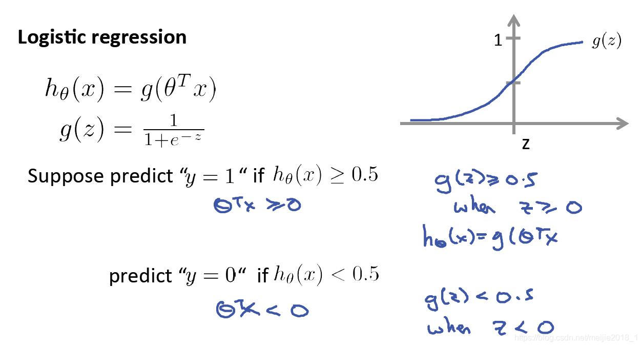
由上图可知，由于最后是要求得y=1的概率，在线性回归的基础上增加了sigmoid函数，将z值映射到区间[0,1]。
当z≥0时，g(z)≥0.5，可以推测y=1，否则y=0。
故其决策边界即为z = theta’*X = 0.
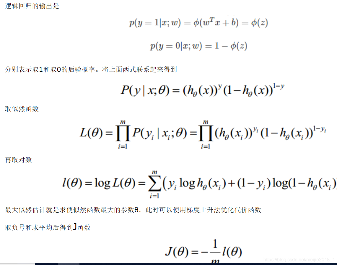
2、代价函数计算

3、matlab编程
（1）原始数据的可视化
补充完整plotData函数，得到图形。

function plotData(X, y)
figure; hold on;
pos = find(y==1);%返回向量y中数值为1的位置,pos也为向量
neg = find(y==0);%返回向量y中数值为0的位置,neg也为向量
%绘制y==1的点，使用红+表示
plot(X(pos,1),X(pos,2),'r+','LineWidth',2,'MarkerSize',7);
%绘制y==0的点，使用蓝o表示
plot(X(neg,1),X(neg,2),'bo','LineWidth',2,'MarkerSize',7);
hold off;
end

在这里插入图片描述
（2）计算代价值和梯度
补充完整sigmoid函数。

function g = sigmoid(z)
g = zeros(size(z));
g = 1./(1+exp(-z));
end

补充完整costFunction函数

function [J, grad] = costFunction(theta, X, y)
m = length(y); % number of training examples
J = 0;
grad = zeros(size(theta));
J = ((log(sigmoid(X*theta)))'*y + (log(1-sigmoid(X*theta)))'*(1-y))/(-m);
grad = (sigmoid(X*theta)-y)'*X/m;
end

计算出theta为零矢量的代价值和梯度分别为：

Cost at initial theta (zeros): 0.693147
Expected cost (approx): 0.693
Gradient at initial theta (zeros): 
 -0.100000 
 -12.009217 
 -11.262842 
Expected gradients (approx):
 -0.1000
 -12.0092
 -11.2628

（3）使用fminunc函数进行优化

options = optimset('GradObj', 'on', 'MaxIter', 400);
[theta, cost] = fminunc(@(t)(costFunction(t, X, y)), initial_theta, options);

% Print theta to screen
fprintf('Cost at theta found by fminunc: %f\n', cost);
fprintf('Expected cost (approx): 0.203\n');
fprintf('theta: \n');
fprintf(' %f \n', theta);
fprintf('Expected theta (approx):\n');
fprintf(' -25.161\n 0.206\n 0.201\n');

Cost at theta found by fminunc: 0.203506
Expected cost (approx): 0.203
theta: 
 -24.933057 
 0.204408 
 0.199619 
Expected theta (approx):
 -25.161
 0.206
 0.201

（4）绘制决策边界

function plotDecisionBoundary(theta, X, y)

plotData(X(:,2:3), y);
hold on;

if size(X, 2) <= 3
    % Only need 2 points to define a line, so choose two endpoints
    plot_x = [min(X(:,2))-2,  max(X(:,2))+2];

    % Calculate the decision boundary line
    plot_y = (-1./theta(3)).*(theta(2).*plot_x + theta(1));

    % Plot, and adjust axes for better viewing
    plot(plot_x, plot_y);
    
    % Legend, specific for the exercise
    legend('Admitted', 'Not admitted', 'Decision Boundary');
    axis([30, 100, 30, 100]);
else
    % Here is the grid range
    u = linspace(-1, 1.5, 50);
    v = linspace(-1, 1.5, 50);

    z = zeros(length(u), length(v));
    % Evaluate z = theta*x over the grid
    for i = 1:length(u)
        for j = 1:length(v)
            z(i,j) = mapFeature(u(i), v(j))*theta;
        end
    end
    z = z'; % important to transpose z before calling contour

    % Plot z = 0
    % Notice you need to specify the range [0, 0]
    contour(u, v, z, [0, 0], 'LineWidth', 2)
end
hold off

end

决策边界在本二元分类中实际为z = theta(1) *x0+ theta(2) *x1 + theta(3) x2 = 0（x0 =1）
解该方程得到 x2 = -1/theta(3)(theta(1) + theta(2) *x1)

获得的图形为：
在这里插入图片描述
（5）预测函数和预测准确率
完成predict函数：

function p = predict(theta, X)
m = size(X, 1); % Number of training examples
p = zeros(m, 1);
p = sigmoid(X*theta) >=0.5;
end

计算数据[1 45 85]分类y = 1的概率：

prob = sigmoid([1 45 85] * theta);
fprintf(['For a student with scores 45 and 85, we predict an admission ' ...
         'probability of %f\n'], prob);
fprintf('Expected value: 0.775 +/- 0.002\n\n');

其输出为：

For a student with scores 45 and 85, we predict an admission probability of 0.774324
Expected value: 0.775 +/- 0.002

统计原始数据分类的准确率：

p = predict(theta, X);
fprintf('Train Accuracy: %f\n', mean(p == y) * 100);
fprintf('Expected accuracy (approx): 89.0\n');
fprintf('\n');

其输出为：

Train Accuracy: 89.000000
Expected accuracy (approx): 89.0

吴恩达机器学习训练2：Logistic回归

猜你喜欢