SVM图像分类步骤:
1,划分数据集
2,图像数据集去均值化处理
对图像的理解:图像中的每一个像素点都相当于一个特征,每一个图像相当于在这个空间中的一个点;去均值化为了避免噪声等影响;SVM采用W正则化目的使得每个维度特征尽可能保留。
3,定义损失函数Loss
对于损失函数的理解:
定义为计算出的每类得分:


w有几行,最后就会输出几个类别的得分。(然而,这样一次只能计算一张图片与其各自类别得分;因此,在cs231n实际计算中涉及到了将W转置,并且将数据集Xi变为行向量,以便于处理庞大的数据集数目)。
例如:
input:
数据集X_train(N,D),数据集标签:y_train(N,),权重W矩阵:(D,C),C:训练数据集中类别的数目(对于Cifar10就为10类即C=10)
举例:之前利用loadCifar读取数据集:
X_train(1000,32,32,3)形式,[即有1000个样本(图片),每个图像32行,32列,并有3个color chanel],先将其预处理,转换为(1000,32*32*3)即(1000,3072),但是计算时增加了一维偏置项,即为X_train(1000,3073),W(3073,10)。
最后计算为:可见上面公式计算得分为:;但是实际代码计算的顺序为:sj=X_train*W,只是影响了在矩阵中的表达顺序,以便更加方便地进行向量化计算,最后输出为y(1000,10),即每一个数据都计算出了其10类中每一个类别的得分。
示例:
-------------------------------------------------------------------------------
ni为图像编号,pi为该图像展开行向量像素值
|      X      ×           W           =     score     |
-------------------------------------------------------------------------------
    p1  p2  p3                            cat     duck      frog
n1  |10  14  10  1|   |0.1  0.2  0.2 |    8.8     [7.2]     4.4  -->第一个样本得分
n2  |5   10  8   1| × |0.2  0.3  0.1 |=   6.5      4.8      2.8  -->第二个样本得分
n3  |10  5   5   1|   |0.5  0.1  0.1 |    4.5      4.0      3.0  -->第三个样本得分
                  bias|0.0  0.0  0.0 |
计算hinge-loss:
其中,是训练集的数据量。现在正则化惩罚添加到了损失函数里面,并用超参数
来计算其权重。该超参数(超参数:即算法执行之前需要预先指定的参数;区别于模型参数:利用算法训练得到的参数。)无法简单确定,需要通过交叉验证来获取。
对于每一个图像都为其分类得到每一个类的得分(有点类似softmax,但softmax是进行求e指数得概率,而这里是直接得出得分),然后利用得分计算损失函数,即折页损失函数(hinge loss)。在后面的作业里面有继续对其损失改进,即增加softmax来对损失结果进行计算。
4,给定权重初始值
因为最开始的w是随机生成的很小的值(注意,这样做是有原因的,因为若w都大致为0,那么第一步计算出的score矩阵的每一个元素也约等于0。
5,梯度下降求最优化问题
整个实现过程,最难理解的地方我个人觉得是该损失函数的梯度是如何实现并进行计算的?
权重更新过程:
【看了一些博客与代码之后有种感觉,权重更新计算过程和感知器算法相似,只是在判断条件上有点差异,主要原因我觉得是由于SVM的损失函数Hinge-loss造成的,因为考虑其性质,max(0,Y),也就是说其对Y的微分(斜率)只有三种取值即:-1,0,1。然后大于零的加,小于零的减。(感知器算法是正确分类的W权重不进行操作,SVM不管分类正确还是错误,都需要对其进行更新;同时感知器算法仅仅以0为分界线,而SVM增加了一个△项,对于损失函数更严格;)】
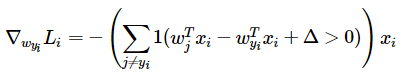
其中的其实就是代码里的判断条件,因为对于max函数而言,结果只能为-1,0,1。
方法一:
循环方式:
def svm_loss_naive(W, X, y, reg):
  """
  Structured SVM loss function, naive implementation (with loops).

  Inputs have dimension D, there are C classes, and we operate on minibatches
  of N examples.

  Inputs:
  - W: A numpy array of shape (D, C) containing weights.
  - X: A numpy array of shape (N, D) containing a minibatch of data.
  - y: A numpy array of shape (N,) containing training labels; y[i] = c means
    that X[i] has label c, where 0 <= c < C.
  - reg: (float) regularization strength

  Returns a tuple of:
  - loss as single float
  - gradient with respect to weights W; an array of same shape as W
  """
  dW = np.zeros(W.shape) # initialize the gradient as zero

  # compute the loss and the gradient
  num_classes = W.shape[1]
  num_train = X.shape[0]
  loss = 0.0
  for i in xrange(num_train):
    scores = X[i].dot(W)
    correct_class_score = scores[y[i]]
    for j in xrange(num_classes):
      if j == y[i]:
        continue
      margin = scores[j] - correct_class_score + 1 # note delta = 1
      if margin > 0:
        loss += margin
        dW[:,y[i]] +=-X[i,:].T
        dW[:,j]+=X[i,:].T

  # Right now the loss is a sum over all training examples, but we want it
  # to be an average instead so we divide by num_train.
  loss /= num_train
  dW  /=num_train

  # Add regularization to the loss.
  loss += reg * np.sum(W * W)
  dW +=reg*W
return loss, dW

##增加了softmax版本

def softmax_loss_naive(W, X, y, reg):

  loss=0.0
  dW=np.zeros_like(W)
  num_classes=W.shape[1]
  num_train=X.shape[0]
  for i in range(num_train):
    scores=X[i].dot(W)
    shift_scores=scores-max(scores)
    loss_i=-shift_scores[y[i]]+np.log(sum(np.exp(shift_scores)))
    loss+=loss_i
    for j in range(num_classes):
      softmax_out=np.exp(shift_scores[j])/sum(np.exp(shift_scores))
      if j==y[i]:
        dW[:,j]+=(-1+softmax_out)*X[i]
      else:
        dW[:,j]+=softmax_out*X[i]
  loss/=num_train
  loss+=0.5*reg*np.sum(W*W)
  dW=dW/num_train+reg*W
  return loss,dW
方法二:
向量形式:
def svm_loss_vectorized(W, X, y, reg):
  """
  Structured SVM loss function, vectorized implementation.

  Inputs and outputs are the same as svm_loss_naive.
  """
  loss = 0.0
  dW = np.zeros(W.shape) # initialize the gradient as zero

  #############################################################################
  # TODO:                                                                     #
  # Implement a vectorized version of the structured SVM loss, storing the    #
  # result in loss.                                                           #
  #############################################################################
  #pass
  scores = X.dot(W)
  num_classes = W.shape[1]
  num_train = X.shape[0]

  scores_correct = scores[np.arange(num_train),y]
  scores_correct = np.reshape(scores_correct,(num_train,-1))
  margins = scores - scores_correct+1
  margins = np.maximum(0,margins)
  margins[np.arange(num_train),y]=0
  loss += np.sum(margins)/num_train
  loss +=0.5*reg*np.sum(W*W)
  #############################################################################
  #                             END OF YOUR CODE                              #
  #############################################################################


  #############################################################################
  # TODO:                                                                     #
  # Implement a vectorized version of the gradient for the structured SVM     #
  # loss, storing the result in dW.                                           #
  #                                                                           #
  # Hint: Instead of computing the gradient from scratch, it may be easier    #
  # to reuse some of the intermediate values that you used to compute the     #
  # loss.                                                                     #
  #############################################################################
  #pass
  margins[margins >0] =1
  row_sum = np.sum(margins,axis =1)
  margins[np.arange(num_train),y] = -row_sum
  dW +=np.dot(X.T,margins)/num_train +reg*W
  #############################################################################
  #                             END OF YOUR CODE                              #
  #############################################################################

  return loss, dW


##增加了softmax版本

def softmax_loss_vectorized(W, X, y, reg):
  loss=0.0
  dW=np.zeros_like(W)
  num_classes=W.shape[1]
  num_train=X.shape[0]
  scores=X.dot(W)

  shift_scores=scores-np.max(scores,axis=1).reshape(-1,1) #先转成(N,1) numpy广播机制 softmax_output=np.exp(shift_scores)/np.sum(np.exp(shift_scores),axis=1).reshape((-1,1))
  softmax_output=np.exp(shift_scores)/np.sum(np.exp(shift_scores),axis=1).reshape((-1,1))

  loss=-np.sum(np.log(softmax_output[range(num_train),list(y)])) #softmax_output[range(num_train),list(y)]计算的是正确分类y_i的损 loss/=num_train
  loss/=num_train
  loss+=0.5*reg*np.sum(W*W)

  dS=softmax_output.copy()
  dS[range(num_train),list(y)]+=-1
  dW=(X.T).dot(dS)
  dW=dW/num_train+reg*W
  return loss,dW
程序执行结果:
完整程序GitHub:https://github.com/TakumiWzy/cs231n_Classifier
wdir='F:/pythonwork/cs231n/cs231n_svmClassifier')
Training data shape:  (50000, 32, 32, 3)
Training labels shape:  (50000,)
Test data shape:  (10000, 32, 32, 3)
Test labels shape:  (10000,)
Train data shape:  (49000, 32, 32, 3)
Train labels shape:  (49000,)
Validation data shape:  (1000, 32, 32, 3)
Validation labels shape:  (1000,)
Test data shape:  (1000, 32, 32, 3)
Test labels shape:  (1000,)
Development data shape:  (500, 32, 32, 3)
Development label shape:  (500,)
Training data shape:  (49000, 3072)
Validation data shape:  (1000, 3072)
Test data shape:  (1000, 3072)
dev data shape:  (500, 3072)
(3072,)
[130.64189796 135.98173469 132.47391837 130.05569388 135.34804082
 131.75402041 130.96055102 136.14328571 132.47636735 131.48467347]
49000
添加偏置项后数据形状为: (49000, 3073) (1000, 3073) (1000, 3073) (500, 3073)
loss: 8.702267
numerical: -4.638723 analytic: -4.638723, relative error: 3.151537e-11
numerical: -2.141041 analytic: -2.141041, relative error: 5.432118e-11
numerical: -11.021807 analytic: -11.021807, relative error: 3.522074e-11
numerical: -9.445677 analytic: -9.445677, relative error: 2.063717e-11
numerical: 13.629505 analytic: 13.732026, relative error: 3.746906e-03
numerical: 8.917645 analytic: 8.917645, relative error: 4.886022e-11
numerical: 2.432030 analytic: 2.432030, relative error: 1.411299e-11
numerical: -6.988180 analytic: -7.023490, relative error: 2.520104e-03
numerical: -10.473082 analytic: -10.473082, relative error: 6.580678e-12
numerical: -7.952713 analytic: -7.952713, relative error: 1.155288e-11
numerical: -4.123088 analytic: -4.120145, relative error: 3.569502e-04
numerical: 17.500421 analytic: 17.531041, relative error: 8.740799e-04
numerical: -43.700488 analytic: -43.677175, relative error: 2.668027e-04
numerical: 9.795672 analytic: 9.801494, relative error: 2.970627e-04
numerical: 15.901370 analytic: 15.895540, relative error: 1.833279e-04
numerical: -12.766090 analytic: -12.762609, relative error: 1.363728e-04
numerical: -1.678366 analytic: -1.681589, relative error: 9.592278e-04
numerical: -10.255365 analytic: -10.255658, relative error: 1.430935e-05
numerical: -24.958209 analytic: -24.954298, relative error: 7.836278e-05
numerical: -14.679750 analytic: -14.681386, relative error: 5.569291e-05
Naive loss: 8.702267e+00 computed in 0.099929s
Vectorized loss: 8.702267e+00 computed in 0.626333s
difference: 0.000000
Naive loss and gradient: computed in 0.105718s
Vectorized loss and gradient: computed in 0.003994s
difference: 0.000000
iteration 0 / 1500: loss 403.653368
iteration 100 / 1500: loss 240.143235
iteration 200 / 1500: loss 145.797747
iteration 300 / 1500: loss 90.220245
iteration 400 / 1500: loss 55.338267
iteration 500 / 1500: loss 35.699744
iteration 600 / 1500: loss 23.384158
iteration 700 / 1500: loss 15.926592
iteration 800 / 1500: loss 11.170984
iteration 900 / 1500: loss 9.019268
iteration 1000 / 1500: loss 7.735003
iteration 1100 / 1500: loss 6.821824
iteration 1200 / 1500: loss 6.764999
iteration 1300 / 1500: loss 5.369674
iteration 1400 / 1500: loss 5.438837
That took 6.372856s
training accuracy: 0.379755
validation accuracy: 0.386000
lr 1.000000e-07 reg 2.500000e+04 train accuracy: 0.331306 val accuracy: 0.336000
lr 1.000000e-07 reg 5.000000e+04 train accuracy: 0.359694 val accuracy: 0.344000
lr 5.000000e-05 reg 2.500000e+04 train accuracy: 0.137694 val accuracy: 0.165000
lr 5.000000e-05 reg 5.000000e+04 train accuracy: 0.043388 val accuracy: 0.040000
best validation accuracy achieved during cross-validation: 0.344000
linear SVM on raw pixels final test set accuracy: 0.350000
参考文章:
https://www.cnblogs.com/Holly-blog/p/8882944.html
https://zhuanlan.zhihu.com/p/20945670?refer=intelligentunit
https://blog.csdn.net/alexxie1996/article/details/79184596#commentBox