波士顿房价预测-ElasticNet模型

lasso/ridge模型分析，即L1-norm/L2-norm
https://blog.csdn.net/weixin_42567027/article/details/107478595

模型介绍

ElasticNet又叫弹性网络回归，也就是L1-norm与L2-norm的组合。

数据集

代码

// An highlighted block
import numpy as np
import matplotlib as mpl
import matplotlib.pyplot as plt
import pandas as pd
##数据分割为训练数据和测试数据
from sklearn.model_selection import train_test_split
#使用ElasticNet模型
from sklearn.linear_model import ElasticNetCV
import sklearn.datasets
from pprint import pprint
#数据预处理
from sklearn.preprocessing import PolynomialFeatures, StandardScaler
from sklearn.pipeline import Pipeline
from sklearn.metrics import mean_squared_error
import warnings

if __name__ == "__main__":

    '''加载数据'''
    #warnings.filterwarnings(action='ignore')
    ##设置浮点精度
    np.set_printoptions(suppress=True)
    #读取数据
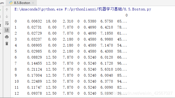
    file_data = pd.read_csv('F:\pythonlianxi\housing.data', header=None)
    #print(file_data)
    # a = np.array([float(s) for s in str if s != ''])

    #将数据分为两部分，并赋值
    #将data设为维度为(len(file_data), 14)的值
    data = np.empty((len(file_data), 14))
    data = sklearn.datasets.load_boston()
    #print(data)
    x = np.array(data.data)
    y = np.array(data.target)
    print (u'样本个数：%d, 特征个数：%d' % x.shape)
    print (y.shape)
    y = y.ravel()
    # #

    '''训练集，测试集，训练模型'''
    #数据分为训练集和测试集
    x_train, x_test, y_train, y_test = train_test_split(x, y, train_size=0.7, random_state=0)
    #线性分类
    model = Pipeline([
        ('ss', StandardScaler()),
        #ElasticNet回归
        ('poly', PolynomialFeatures(degree=3, include_bias=True)),
        ('linear', ElasticNetCV(l1_ratio=[0.1, 0.3, 0.5, 0.7, 0.99, 1], alphas=np.logspace(-3, 2, 5),
                                fit_intercept=False, max_iter=1e3, cv=3))
    ])
    print (u'开始建模...')
    #拟合模型
    model.fit(x_train, y_train)
    #获得模型的参数
    linear = model.get_params('linear')['linear']
    print (u'超参数：', linear.alpha_)
    print (u'L1 ratio：', linear.l1_ratio_)
    #argsort的：对数据进行排序，然后提取其原来的索引
    #测试数据做递增排序
    order = y_test.argsort(axis=0)
    y_test = y_test[order]
    x_test = x_test[order, :]
    #使用测试数据测试模型
    y_pred = model.predict(x_test)

    '''计算R2，MSE'''
    #为模型进行打分 r2越大，拟合效果越好，最优值为1。
    r2 = model.score(x_test, y_test)
    #计算MSE
    mse = mean_squared_error(y_test, y_pred)
    print ('R2:', r2)
    print( u'均方误差：', mse)
    #t：样本标号
    t = np.arange(len(y_pred))

    '''绘图'''
    mpl.rcParams['font.sans-serif'] = [u'simHei']
    mpl.rcParams['axes.unicode_minus'] = False
    plt.figure(facecolor='w')
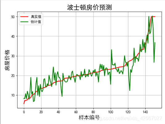
    plt.plot(t, y_test, 'r-', lw=2, label=u'真实值')
    plt.plot(t, y_pred, 'g-', lw=2, label=u'估计值')
    plt.legend(loc='best')
    plt.title(u'波士顿房价预测', fontsize=18)
    plt.xlabel(u'样本编号', fontsize=15)
    plt.ylabel(u'房屋价格', fontsize=15)
    plt.grid()
    plt.show()

实验结果

超参数： 0.01778279410038923
L1 ratio： 0.99
均方误差： 16.125736558067832