原文:https://medium.com/dissecting-bert/dissecting-bert-part-1-d3c3d495cdb3
A meaningful representation of the input, you must encode
This is Part 1/2 of Dissecting BERT written by Miguel Romero and Francisco Ingham. Each article was written jointly by both authors. If you already understand the Encoder architecture from Attention is All You Need and you are interested in the differences that make BERT awesome, head on to BERT Specifics.
这是Miguel Romero和Francisco Ingham撰写的解剖BERT的第1/2部分。每篇文章都是由两位作者共同撰写的。如果您已经了解了“Attention is All You Need”编码器架构,并且您对使BERT非常棒的原因感兴趣,请转向BERT细节。
Many thanks to Yannet Interian for her revision and feedback.
In this blog post, we are going to examine the Encoder architecture in depth (see Figure 1) as described in Attention Is All You Need. In BERT Specifics we will dive into the novel modifications that make BERT particularly effective.
在这篇博文中,我们将深入研究编码器架构(参见图1),如“Attention Is All You Need”中所述。在BERT细节中,我们将深入探讨使BERT特别有效的新颖修改。
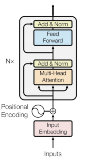
Figure 1: The Encoder
Notation
Before we begin, let’s define the notation we will use throughout the article:
emb_dim: Dimension of the token embeddings.
词嵌入维度
input_length: Length of the input sequence (the same in all sequences in a specific batch due to padding).
输入序列的长度(由于相同batch中会使用padding,所有序列会有相同的长度)
hidden_dim: Size of the Feed-Forward network’s hidden layer.
前馈网络隐藏层的大小
vocab_size: Amount of words in the vocabulary (derived from the corpus).
词典中的单词数量(来自语料库)。
Introduction
The Encoder used in BERT is an attention-based architecture for Natural Language Processing (NLP) that was introduced in the paper Attention Is All You Need a year ago. The paper introduces an architecture called the Transformer which is composed of two parts, the Encoder and the Decoder. Since BERT only uses the Encoder we are only going to explain that in this blog post (if you want to learn about the Decoder and how it is integrated with the Encoder, we wrote a separate blog post on this).
BERT中使用的encoder是一种基于注意力的自然语言处理(NLP)架构,它在一年前的Attention Is All You Need一文中引入。本文介绍了一种称为transformer的架构,它由两部分组成,即编码器和解码器。由于BERT只使用编码器,我们只会在这篇博文中解释一下(如果你想了解解码器以及它如何与编码器集成,我们就此写了一篇单独的博客文章)。
Transfer learning has quickly become a standard for state of the art results in NLP since the release of ULMFiT earlier this year. After that, remarkable advances have been achieved by combining the Transformer with transfer learning. Two iconic examples of this combination are OpenAI’s GPT and Google AI’s BERT.
自今年早些时候ULMFiT发布以来,迁移学习已迅速成为NLP最先进成果的标准。之后,通过将T与迁移学习相结合,取得了显着的进步。这种组合的两个标志性例子是OpenAI的GPT和Google AI的BERT。
This series aims to:
- Provide an intuitive understanding of the Transformer and BERT’s underlying architecture.
- Explain the fundamental principles of what makes BERT so successful in NLP tasks.
- 提供对Transformer和BERT底层架构的直观理解。
- 解释使BERT在NLP任务中如此成功的基本原理。
To explain this architecture we will adopt the general to specifics approach. We will start by looking at the information flow in the architecture and we will dive into the inputs and outputs of the Encoder as presented in the paper. Next, we will look into each of the encoder blocks and understand how Multi-Head Attention is used. Don't worry if you don't know what that is yet; we will make sure you understand it by the end of this article.
为了解释这种架构,我们将采用一般到具体的方法。我们将从查看架构中的信息流开始,我们将深入研究编码器中的输入和输出。接下来,我们将查看每个编码器块并了解如何使用多头注意。如果你不知道那是什么,别担心;我们将确保您在本文结尾处理解它。
Information Flow
The data flow through the architecture is as follows:
- The model represents each token as a vector of emb_dim size. With one embedding vector for each of the input tokens, we have a matrix of dimensions (input_length) x (emb_dim) for a specific input sequence.
- It then adds positional information (positional encoding). This step returns a matrix of dimensions (input_length) x (emb_dim), just like in the previous step.
- The data goes through N encoder blocks. After this, we obtain a matrix of dimensions (input_length) x (emb_dim).
- 该模型将每个单词表示为emb_dim大小的向量。对于每个输入单词使用一个嵌入向量,我们将获得一个特定输入序列的矩阵,维度是(input_length)x(emb_dim)。
- 然后对它添加位置信息(位置编码)。此步骤返回维度矩阵(input_length)x(emb_dim),就像上一步骤一样。
- 数据通过N个编码器块。在此之后,我们获得的矩阵维度仍然是是(input_length)x(emb_dim)。
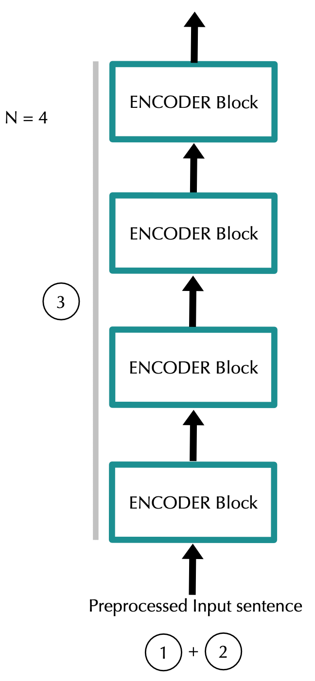
Figure 2: Information flow in the Encoder
Note: The dimensions of the input and output of the encoder block are the same. Hence, it makes sense to use the output of one encoder block as the input of the next encoder block.
编码器块的输入和输出的尺寸相同。因此,使用一个编码器块的输出作为下一个编码器块的输入是有意义的。
Note: In BERT's experiments, the number of blocks N (or L, as they call it) was chosen to be 12 and 24.
在BERT的实验中,块数N(或L,他们称之为)被选择为12和24。
Note: The blocks do not share weights with each other
这些块彼此不共享权重
From words to vectors
Tokenization, numericalization and word embeddings
单词化,数字化和词嵌入
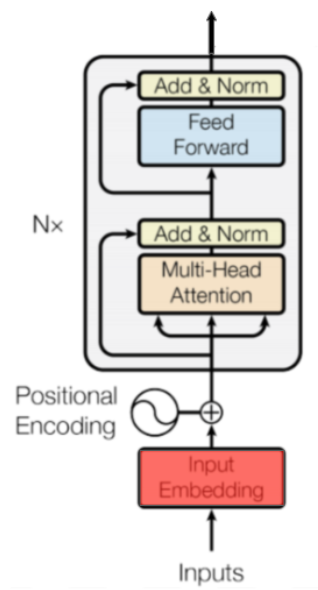
Figure 3: Where tokenization, numericalization and embeddings happen.
Tokenization, numericalization and embeddings do not differ from the way it is done with RNNs. Given a sentence in a corpus:
标记化,数字化和嵌入与使用RNN的方式没有区别。比如语料库中的句子:
“ Hello, how are you?”
The first step is to tokenize it:
第一步是将其拆开:
“ Hello, how are you?” → [“Hello”, “,” , “how”, “are”, “you”, “?”]
This is followed by numericalization, mapping each token to a unique integer in the corpus’ vocabulary.
然后进行数值化,将每个标记映射到语料库词汇表中的唯一整数。
[“Hello”, “, “, “how”, “are”, “you”, “?”] → [34, 90, 15, 684, 55, 193]
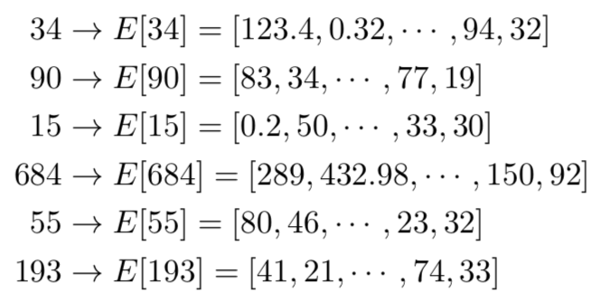
Next, we get the embedding for each word in the sequence. Each word of the sequence is mapped to a emb_dim dimensional vector that the model will learn during training. You can think about it as a vector look-up for each token. The elements of those vectors are treated as model parameters and are optimized with back-propagation just like any other weights.
接下来,我们得到序列中每个单词的嵌入。序列中的每个单词都映射到模型将在训练期间学习的emb_dim维向量。您可以将其视为查找每个token的向量。这些矢量的元素被视为模型参数,并且与任何其他权重一样,使用反向传播进行优化。
Therefore, for each token, we look up the corresponding vector:
因此,对于每个令牌,我们查找相应的向量:
Stacking each of the vectors together we obtain a matrix Z of dimensions (input_length) x (emb_dim):
将每个向量堆叠在一起,我们得到一个维度为(input_length)x(emb_dim)的矩阵Z:
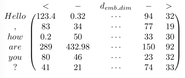
It is important to remark that padding was used to make the input sequences in a batch have the same length. That is, we increase the length of some of the sequences by adding ‘<pad>’ tokens. The sequence after padding might be:
值得注意的是同一个batch中需要保证所有句子又相同的长度。也就是说,我们通过添加'<pad>'标记来增加某些序列的长度。填充后的序列可能是:
[“<pad>”, “<pad>”, “<pad>”, “Hello”, “, “, “how”, “are”, “you”, “?”] → [5, 5, 5, 34, 90, 15, 684, 55, 193]
if the input_length was set to 9.
如果input_length设置为9。
Positional Encoding
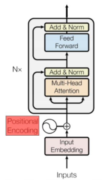
Figure 4: Where Positional Encoding is computed.
Note: In BERT the authors used learned positional embeddings. If you are only interested in BERT you can skip this section where we explain the functions used to calculate the positional encodings in Attention is All You Need
注意:在BERT中,作者使用了学习好的位置嵌入。如果您只对BERT感兴趣,可以跳过本节,我们将在Attention is All You Need中解释用于计算位置编码的函数。
At this point, we have a matrix representation of our sequence. However, these representations are not encoding the fact that words appear in different positions.
此时,我们有一个矩阵表示我们的序列。然而,这些表示并不能体现出编码单词出现在不同位置的事实。
Intuitively, we aim to be able to modify the represented meaning of a specific word depending on its position. We don't want to change the full representation of the word but we want to modify it a little to encode its position.
直观地,我们的目标是能够根据其位置修改单词的representation。但是只想稍微修改它使他能带上位置信息而不是彻底对representation改头换面。
The approach chosen in the paper is to add numbers between [-1,1] using predetermined (non-learned) sinusoidal functions to the token embeddings. Observe that now, for the rest of the Encoder, the word will be represented slightly differently depending on the position the word is in (even if it is the same word).
本文选择的方法是使用预定(非学习)正弦函数将[-1,1]之间的数字加到词嵌入中。现在观察一下,对于编码器的其余部分,根据单词所处的位置(即使它是同一个单词),单词的表示会略有不同。
Moreover, we would like the Encoder to be able to use the fact that some words are in a given position while, in the same sequence, other words are in other specific positions. That is, we want the network to able to understand relative positions and not only absolute ones. The sinuosidal functions chosen by the authors allow positions to be represented as linear combinations of each other and thus allow the network to learn relative relationships between the token positions.
此外,我们希望编码器能够使用这样的事实:某些单词处于给定位置,而在同一序列中,其他单词处于其他特定位置。也就是说,我们希望网络能够理解相对位置而不仅仅是绝对位置。作者选择的sinuosidal函数允许位置表示为彼此的线性组合,从而允许网络学习令牌位置之间的相对关系。
The approach chosen in the paper to add this information is adding to Z a matrix P with positional encodings.
Z + P
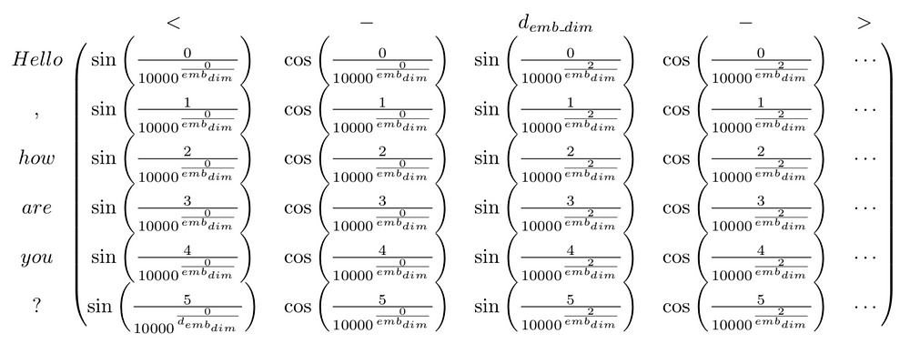
The authors chose to use a combination of sinusoidal functions. Mathematically, using i for the position of the token in the sequence and j for the position of the embedding feature:
作者选择使用正弦函数的组合。在数学上,使用i作为序列中令牌的位置,使用j作为嵌入特征的位置:
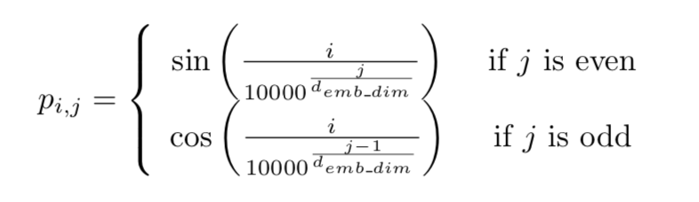
More specifically, for a given sentence P, the positional embedding matrix would be as follows:
更具体地,对于给定的句子P,位置嵌入矩阵将如下:
The authors explain that the result of using this deterministic method instead of learning positional representations (just like we did with the tokens) lead to similar performance. Moreover, this approach had some specific advantages over learned positional representations:
作者解释说,使用这种确定性方法而不是通过网络去学习位置表示(就像我们对令牌所做的那样)可以有相似的性能。此外,这种方法比学习的位置表示具有一些特定的优势:
- The input_length can be increased indefinitely since the functions can be calculated for any arbitrary position.
- Fewer parameters needed to be learned and the model trained quicker.
input_length可以无限增加,因为可以为任意位置计算函数。
需要学习的参数更少,模型训练更快。
The resulting matrix:
X = Z + P
is the input of the first encoder block and has dimensions (input_length) x (emb_dim).
是第一个编码器块的输入,并具有维度(input_length)x(emb_dim)。
Encoder block
A total of N encoder blocks are chained together to generate the Encoder’s output. A specific block is in charge of finding relationships between the input representations and encode them in its output.
总共N个编码器块链接在一起以生成编码器的输出。特定块负责查找输入表示之间的关系并在其输出中对它们进行编码。
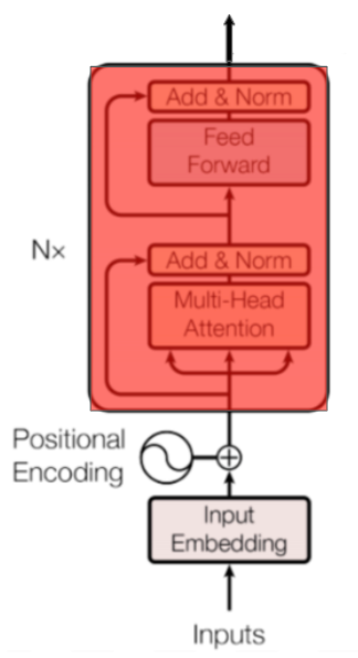
Figure 5: Encoder block.
Intuitively, this iterative process through the blocks will help the neural network capture more complex relationships between words in the input sequence. You can think about it as iteratively building the meaning of the input sequence as a whole.
直观地说,这个通过块的迭代过程将帮助神经网络捕获输入序列中的单词之间更复杂的关系。您可以将其视为迭代地构建输入序列的整体含义。
Multi-Head Attention
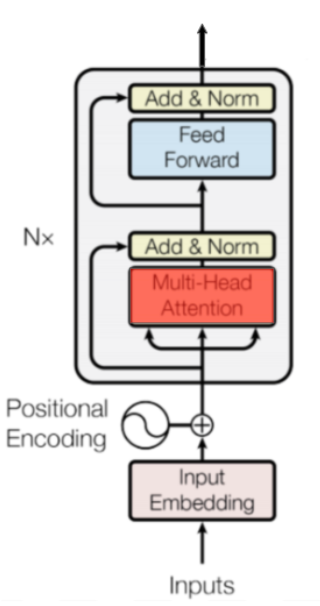
Figure 6: Where Multi-Head Attention happens.
The Transformer uses Multi-Head Attention, which means it computes attention h different times with different weight matrices and then concatenates the results together.
Transformer使用Multi-Head Attention,这意味着它使用不同的权重矩阵计算不同时间的注意力,然后将结果连接在一起。
The result of each of those parallel computations of attention is called a head. We are going to denote a specific head and the associated weight matrices with the subscript i.
每个并行计算注意力的结果称为头部。我们将用下标i表示特定的头部和相关的权重矩阵。
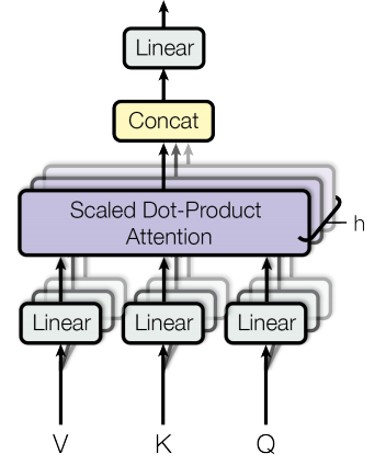
Figure 7: Illustration of the parallel heads computations and their concatenation
As shown in Figure 7, once all the heads have been computed they will be concatenated. This will result in a matrix of dimensions (input_length) x (h*d_v). Afterwards, a linear layer with weight matrix W⁰ of dimensions (h*d_v) x (emb_dim) will be applied leading to a final result of dimensions (input_length) x (emb_dim). Mathematically:
如图7所示,一旦计算了所有头,它们将被连接起来。这将产生维度为(input_length)x(h * d_v)的矩阵。然后,将使用维度是(h * d_v)x(emb_dim)的权重矩阵W'的对其进行线性变换,从而获得的最终结果为(input_length)x(emb_dim):
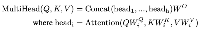
Where Q,K and V are placeholders for different input matrices. In particular, for this case Q,K and V will be replaced by the output matrix of the previous step X.
其中Q,K和V是不同输入矩阵的占位符。特别的,对于这种情况,Q,K和V将被前一步骤X的输出矩阵代替。
Scaled Dot-Product Attention
Overview
Each head is going to be characterized by three different projections (matrix multiplications) given by matrices:
每个head将由三个不同投影矩阵表征:
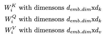
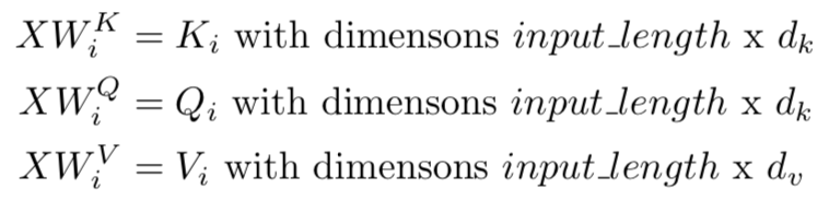
To compute a head we will take the input matrix X and separately project it with the above weight matrices:
为了计算头部,我们将用输入矩阵X分别与上述权重矩阵相乘得到“投影”:
Note: In the paper d_k and d_v are set such that d_k = d_v = emb_dim/h
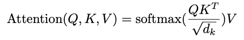
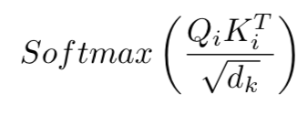
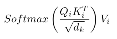
Once we have K_i, Q_i and V_i we use them to compute the Scaled Dot-Product Attention:
一旦我们有了K_i,Q_i和V_i,我们就用它们来计算Scaled Dot-Product Attention:
Graphically:
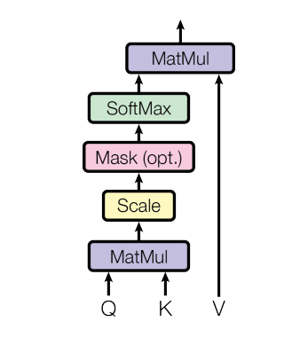
Figure 8: Illustration of the Dot-Product Attention.
Note: In the encoder block the computation of attention does not use a mask. In our Decoder post we explain how the decoder uses masking.
Going Deeper
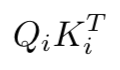
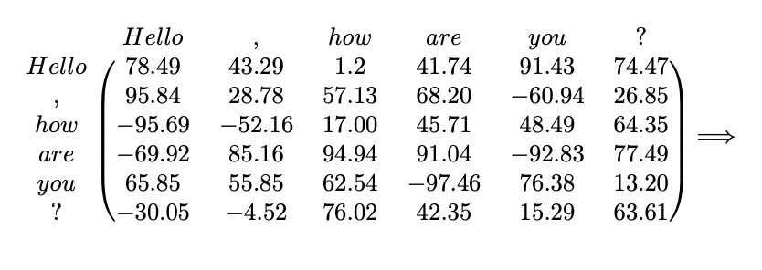
This is the key of the architecture (the name of the paper is no coincidence) so we need to understand it carefully. Let’s start by looking at the matrix product between Q_i and K_i transposed:
下面的公式是架构的关键(论文的名称并非巧合),需要我们仔细理解。让我们从查看Q_i和K_i转置之间的矩阵乘积开始:
Remember that Q_i and K_i were different projections of the tokens into a d_kdimensional space. Therefore, we can think about the dot product of those projections as a measure of similarity between tokens projections. For every vector projected through Q_i the dot product with the projections through K_i measures the similarity between those vectors. If we call v_i and u_j the projections of the i-th token and the j-th token through Q_i and K_i respectively, their dot product can be seen as:
请记住,Q_i和K_i是token在d_k维空间中的不同投影。因此,我们可以考虑这些投影的点积作为标记投影之间相似性的度量。对于通过Q_i投射的每个矢量,与通过K_i投影的矢量进行点积,其结果可以表示这些矢量之间的相似性。如果我们令v_i为第i个token通过Q_i得到的投影,u_j为第j个token通过K_i得到的投影,则它们的点积可以看作:
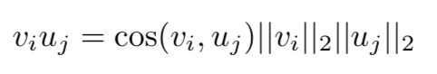
Thus, this is a measure of how similar are the directions of u_i and v_j and how large are their lengths (the closest the direction and the larger the length, the greater the dot product).
因此,这是对u_i和v_j的方向有多相似以及它们的长度有多大的度量(方向越接近,长度越大,点积越大)。
Another way of thinking about this matrix product is as the encoding of a specific relationship between each of the tokens in the input sequence (the relationship is defined by the matrices K_i, Q_i).
该矩阵乘积的意义也可以视为:对输入序列中的每个token之间的特定关系进行编码(该关系由矩阵K_i,Q_i定义)。
After this multiplication, the matrix is divided element-wise by the square root of d_k for scaling purposes.
在该乘法之后,为了缩放目的,矩阵被除以d_k的平方根。
The next step is a Softmax applied row-wise (one softmax computation for each row):
下一步是逐行应用Softmax(每行一次softmax计算):
(注:此时维度(length, dk) dot (dk,length) = (length, length) )
In our example, this could be:
Before Softmax
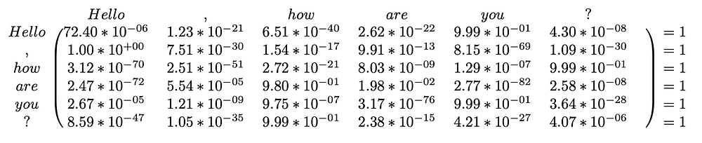
After Softmax
The result would is rows with numbers between zero and one that sum to one. Finally, the result is multiplied by V_i to get the result of the head.
结果是数字在0和1之间的行总和为1。最后,结果乘以V_i得到头部的结果。
Example 1
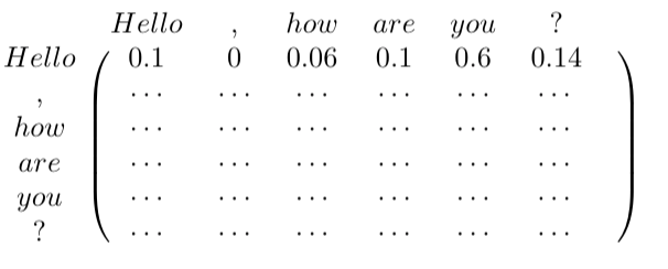
For the sake of understanding let’s propose a dummy example. Suppose that the resulting first row of:
为了便于理解,让我们提出一个虚拟的例子。假设得到的第一行:
is [0,0,0,0,1,0]. Hence, because 1 is in the 5th position of the vector, the result will then be:
是[0,0,0,0,1,0]。因此,因为1位于向量的第5个位置,结果将是:
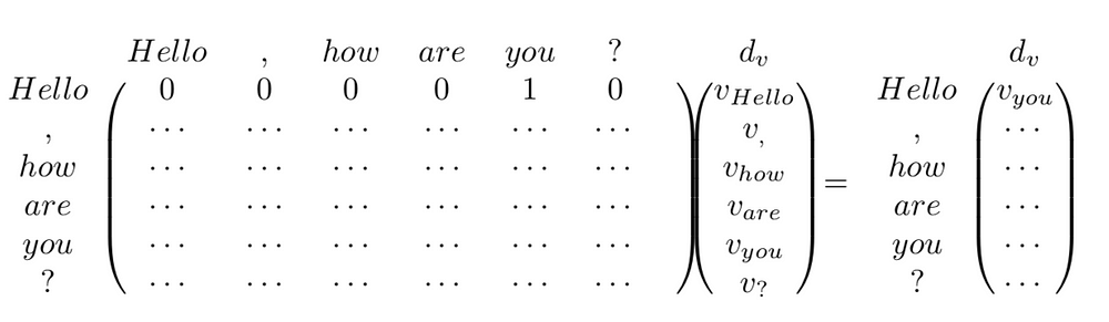
Where v_{token} is the projection through V_i of the token’s representation. Observe that in this case the word “hello” ends up with a representation based on the 4th token “you” of the input for that head.
其中v_ {token}是token在V_i下的投影。注意,在这种情况下,单词“hello”最终会得到一个基于该head的输入的第4个token “you”的表示。
(注:实际上dv是(length, dv)维度的,这里将v_ {token}视作一个dv维度的vector)
Supposing an equivalent example for the rest of the heads. The word “Hello”will be now represented by the concatenation of the different projections of other words. The network will learn over training time which relationships are more useful and will relate tokens to each other based on these relationships.
假设其余头部的也进行类似的过程。 “Hello”一词现在将由不同head得到的投影结果拼接得到。网络将在训练时了解哪些关系(或者说哪些投影)更有用,并加深这种联系。
Example 2
Let us now complicate the example a little bit more. Suppose now our previous example in the more general scenario where there isn’t just a single 1 per row but decimal positive numbers that sum to 1:
现在让我们将这个例子复杂化一点。现在假设我们之前的例子在更一般的场景中,每行不只有一个,而是总和为1的十进制正数:
If we do as in the previous example and multiply that by V_i:
如果我们按照前面的示例执行操作并将其乘以V_i:
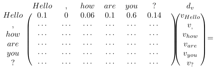
This results in a matrix where each row is a composition of the projection of the token’s representations through V_i:
这会产生一个矩阵,其中每一行都是 token经过V_i投影后的结果的组合:
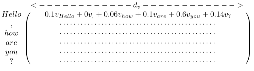
Observe that we can think about the resulting representation of “Hello” as a weighted combination (centroid) of the projected vectors through V_i of the input tokens.
hello的最终表示可以看作所有输入token的加权组合(质心)。
Thus, a specific head captures a specific relationship between the input tokens. Now, if we do that h times (a total of h heads) each encoder block is capturing h different relationships between input tokens.
因此,特定头部捕获输入token之间的特定关系。现在,如果我们这样做h次(总共h个头),每个不同的head就是在捕获输入token之间的不同关系。
Following up, assume that the example above referred to the first head. Then the first row would be:
假设上面的例子引用了第一个头。然后第一行将是:

Then the first row of the result of the Multi-Head Attention layer, i.e. the representation of “Hello” at this point, would be
然后,多头注意层的结果的第一行,即此时“Hello”的表示,将是
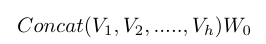
Which is a vector of length emb_dim given that the matrix W_0 has dimensions (d_v*h) x (emb_dim). Applying the same logic in the rest of the rows/tokens representations we obtain a matrix of dimensions (input_length) x (emb_dim).
在给定矩阵W_0具有维度(d_v * h)x(emb_dim)的情况下,将获得长度为emb_dim的向量。在其余的行/标记中应用相同的逻辑,我们获得维度矩阵(input_length)x(emb_dim)。
Thus, at this point, the representation of the token is the concatenation of h weighted combinations of token representations (centroids) through the h different learned projections.
因此,此时,token的表示是通过h个不同的投影的结果的加权组合的拼接。
Position-wise Feed-Forward Network
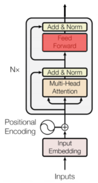
Figure 9: Feed Forward
This step is composed of the following layers:
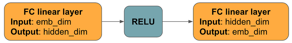
Figure 10: Scheme of the Feed Forwards Neural Netwrok
Mathematically, for each row in the output of the previous layer:
在数学上,对于前一层输出中的每一行:

where W_1 and W_2 are (emb_dim) x (d_F) and (d_F) x (emb_dim) matrices respectively.
Observe that during this step, vector representations of tokens don’t “interact” with each other. It is equivalent to run the calculations row-wise and stack the resulting rows in a matrix.
观察到在此步骤中,token的矢量表示不会彼此“相互作用”。它等效于逐行运行计算并将结果行堆叠在矩阵中。
The output of this step has dimension (input_length) x (emb_dim).
Dropout, Add & Norm
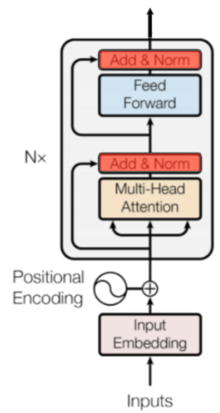
Figure 11: Where Dropout, Addition and normalization happens.
Before this layer, there is always a layer for which inputs and outputs have the same dimensions (Multi-Head Attention or Feed-Forward). We will call that layer Sublayer and its input x.
在此层之前,始终存在一个输入和输出具有相同尺寸的层(多头注意或前馈)。我们将称该层为Sublayer,其输入被称为x。
After each Sublayer, dropout is applied with 10% probability. Call this result Dropout(Sublayer(x)). This result is added to the Sublayer’s input x, and we get x + Dropout(Sublayer(x)).
在每个子层之后,dropout设为10%。调用此结果Dropout(Sublayer(x))。这个结果被添加到Sublayer的输入x,我们得到x + Dropout(Sublayer(x))。
Observe that in the context of a Multi-Head Attention layer, this means adding the original representation of a token x to the representation based on the relationship with other tokens. It is like telling the token:
观察到在多头注意层的上下文中,token的原始表示和混合了与其他token的关系后得到的新表示被加在一起。这就像告诉令牌:
“Learn the relationship with the rest of the tokens, but don’t forget what we already learned about yourself!”
Finally, a token-wise/row-wise normalization is computed with the mean and standard deviation of each row. This improves the stability of the network.
The output of these layers is:
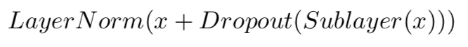
And that’s it! This is the architecture behind all of the magic in state of the art NLP.
If you have any feedback please let us know in the comment section!
References
Attention Is All You Need; Vaswani et al., 2017.
BERT: Pre-training of Deep Bidirectional Transformers for Language Understanding; Devlin et al., 2018.
The Annotated Transformer; Alexander Rush, Vincent Nguyen and Guillaume Klein.
Universal Language Model Fine-tuning for Text Classification; Howard et al., 2018.
Improving Language Understanding by Generative Pre-Training; Radford et al., 2018.
Source of cover picture: Cripttografia e numeri prim