原文:https://jalammar.github.io/illustrated-transformer/
part2:https://blog.csdn.net/zongza/article/details/88866476
In the previous post, we looked at Attention – a ubiquitous method in modern deep learning models. Attention is a concept that helped improve the performance of neural machine translation applications. In this post, we will look at The Transformer – a model that uses attention to boost the speed with which these models can be trained. The Transformers outperforms the Google Neural Machine Translation model in specific tasks. The biggest benefit, however, comes from how The Transformer lends itself to parallelization. It is in fact Google Cloud’s recommendation to use The Transformer as a reference model to use their Cloud TPU offering. So let’s try to break the model apart and look at how it functions.
The Transformer was proposed in the paper Attention is All You Need. A TensorFlow implementation of it is available as a part of the Tensor2Tensor package. Harvard’s NLP group created a guide annotating the paper with PyTorch implementation. In this post, we will attempt to oversimplify things a bit and introduce the concepts one by one to hopefully make it easier to understand to people without in-depth knowledge of the subject matter.
A High-Level Look
Let’s begin by looking at the model as a single black box. In a machine translation application, it would take a sentence in one language, and output its translation in another.
首先将这个模型看成是一个黑箱操作。在机器翻译中,就是输入一种语言,输出另一种语言。
![]()
Popping open that Optimus Prime goodness, we see an encoding component, a decoding component, and connections between them.
那么拆开这个黑箱,我们可以看到它是由编码组件、解码组件和它们之间的连接组成。
![]()
The encoding component is a stack of encoders (the paper stacks six of them on top of each other – there’s nothing magical about the number six, one can definitely experiment with other arrangements). The decoding component is a stack of decoders of the same number.
编码组件部分由一堆编码器(encoder)构成(论文中是将6个编码器叠在一起——数字6没有什么神奇之处,你也可以尝试其他数字)。解码组件部分也是由相同数量(与编码器对应)的解码器(decoder)组成的。
![]()
The encoders are all identical in structure (yet they do not share weights). Each one is broken down into two sub-layers:
所有的编码器在结构上都是相同的,但它们没有共享参数。每个解码器都可以分解成两个子层。
![]()
The encoder’s inputs first flow through a self-attention layer – a layer that helps the encoder look at other words in the input sentence as it encodes a specific word. We’ll look closer at self-attention later in the post.
The outputs of the self-attention layer are fed to a feed-forward neural network. The exact same feed-forward network is independently applied to each position.
The decoder has both those layers, but between them is an attention layer that helps the decoder focus on relevant parts of the input sentence (similar what attention does in seq2seq models).
从编码器输入的句子首先会经过一个自注意力(self-attention)层,这层帮助编码器在对每个单词编码时关注输入句子的其他单词。我们将在稍后的文章中更深入地研究自注意力。(注: 按照我的理解,self att的作用就是在编码某个单词的时候同时考虑到句子里的其他单词的影响,也就是所谓的dependency)
自注意力层的输出会传递到前馈(feed-forward)神经网络中。每个位置的单词对应的前馈神经网络都完全一样(注:另一种解读就是一层窗口为一个单词的一维卷积神经网络)。
解码器中也有编码器的自注意力(self-attention)层和前馈(feed-forward)层。除此之外,这两个层之间还有一个注意力层,用来关注输入句子的相关部分(注: 和seq2seq模型的注意力作用相似,作用是用decoder的当前时间步产生的query向量从encoder的特征序列中取出来想要的部分内容)。
![]()
Bringing The Tensors Into The Picture
Now that we’ve seen the major components of the model, let’s start to look at the various vectors/tensors and how they flow between these components to turn the input of a trained model into an output.
我们已经了解了模型的主要部分,接下来我们看一下各种向量或张量(译注:张量概念是矢量概念的推广,可以简单理解矢量是一阶张量、矩阵是二阶张量。)是怎样在模型的不同部分中,将输入转化为输出的。
As is the case in NLP applications in general, we begin by turning each input word into a vector using an embedding algorithm.
像大部分NLP应用一样,我们首先将每个输入单词通过词嵌入算法转换为词向量。
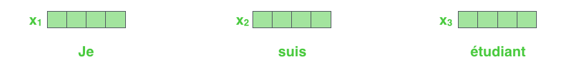
Each word is embedded into a vector of size 512. We'll represent those vectors with these simple boxes.
每个单词都被嵌入为512维的向量,我们用这些简单的方框来表示这些向量。
The embedding only happens in the bottom-most encoder. The abstraction that is common to all the encoders is that they receive a list of vectors each of the size 512 – In the bottom encoder that would be the word embeddings, but in other encoders, it would be the output of the encoder that’s directly below. The size of this list is hyperparameter we can set – basically it would be the length of the longest sentence in our training dataset.
词嵌入过程只发生在最底层的编码器中。所有的编码器都有一个相同的特点,即它们接收一个向量列表,列表中的每个向量大小为512维。在底层(最开始)编码器中它就是词向量,但是在其他编码器中,它就是下一层编码器的输出(也是一个向量列表)。向量列表大小是我们可以设置的超参数——一般是我们训练集中最长句子的长度。
After embedding the words in our input sequence, each of them flows through each of the two layers of the encoder.
将输入序列进行词嵌入之后,每个单词都会流经编码器中的两个子层。
Here we begin to see one key property of the Transformer, which is that the word in each position flows through its own path in the encoder. There are dependencies between these paths in the self-attention layer. The feed-forward layer does not have those dependencies, however, and thus the various paths can be executed in parallel while flowing through the feed-forward layer.
接下来我们看看Transformer的一个核心特性,在这里输入序列中每个位置的单词在编码器中都有自己独特的flow路径。在自注意力层中,这些路径之间存在依赖关系。而前馈(feed-forward)层没有这些依赖关系。因此在前馈(feed-forward)层时可以并行执行各种路径。
Next, we’ll switch up the example to a shorter sentence and we’ll look at what happens in each sub-layer of the encoder.
然后我们将以一个更短的句子为例,看看编码器的每个子层中发生了什么。
Now We’re Encoding!
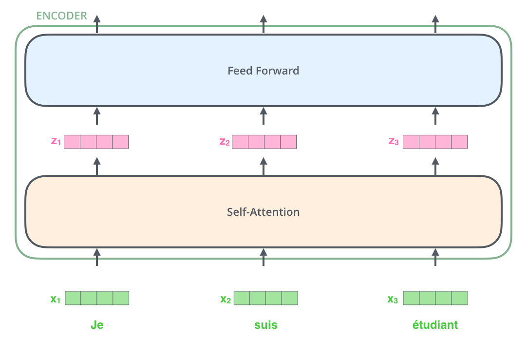
As we’ve mentioned already, an encoder receives a list of vectors as input. It processes this list by passing these vectors into a ‘self-attention’ layer, then into a feed-forward neural network, then sends out the output upwards to the next encoder.
如上述已经提到的,一个编码器接收向量列表作为输入,接着将向量列表中的向量传递到自注意力层进行处理,然后传递到前馈神经网络层中,将输出结果传递到下一个编码器中。
The word at each position passes through a self-encoding process. Then, they each pass through a feed-forward neural network -- the exact same network with each vector flowing through it separately.
输入序列的每个单词都经过自编码过程。然后,他们各自通过前向传播神经网络(每个向量都分别通过,相当于共享这个MLP的参数)
Self-Attention at a High Level
Don’t be fooled by me throwing around the word “self-attention” like it’s a concept everyone should be familiar with. I had personally never came across the concept until reading the Attention is All You Need paper. Let us distill how it works.
不要被我用自注意力这个词弄迷糊了,好像每个人都应该熟悉这个概念。其实我之也没有见过这个概念,直到读到Attention is All You Need 这篇论文时才恍然大悟。让我们精炼一下它的工作原理。
Say the following sentence is an input sentence we want to translate:
例如,下列句子是我们想要翻译的输入句子:
”The animal didn't cross the street because it was too tired”
What does “it” in this sentence refer to? Is it referring to the street or to the animal? It’s a simple question to a human, but not as simple to an algorithm.
这个“it”在这个句子是指什么呢?它指的是street还是这个animal呢?这对于人类来说是一个简单的问题,但是对于算法则不是。
When the model is processing the word “it”, self-attention allows it to associate “it” with “animal”.
当模型处理这个单词“it”的时候,自注意力机制会允许“it”与“animal”建立联系。
As the model processes each word (each position in the input sequence), self attention allows it to look at other positions in the input sequence for clues that can help lead to a better encoding for this word.
随着模型处理输入序列的每个单词,自注意力会关注整个输入序列的所有单词,帮助模型对本单词更好地进行编码。
If you’re familiar with RNNs, think of how maintaining a hidden state allows an RNN to incorporate its representation of previous words/vectors it has processed with the current one it’s processing. Self-attention is the method the Transformer uses to bake the “understanding” of other relevant words into the one we’re currently processing.
如果你熟悉RNN(循环神经网络),回忆一下它是如何维持隐藏层的。RNN会将它已经处理过的前面的所有单词/向量的表示与它正在处理的当前单词/向量结合起来。而自注意力机制会将所有相关单词的理解融入到我们正在处理的单词中。
![]()
As we are encoding the word "it" in encoder #5 (the top encoder in the stack), part of the attention mechanism was focusing on "The Animal", and baked a part of its representation into the encoding of "it".
当我们在编码器#5(栈中最上层编码器)中编码“it”这个单词的时,注意力机制的部分会去关注“The Animal”,将它的表示的一部分编入“it”的编码中。
Be sure to check out the Tensor2Tensor notebook where you can load a Transformer model, and examine it using this interactive visualization.
请务必检查Tensor2Tensor notebook ,在里面你可以下载一个Transformer模型,并用交互式可视化的方式来检验。
Self-Attention in Detail
Let’s first look at how to calculate self-attention using vectors, then proceed to look at how it’s actually implemented – using matrices.
首先我们了解一下如何使用向量来计算自注意力,然后来看它实怎样用矩阵来实现。
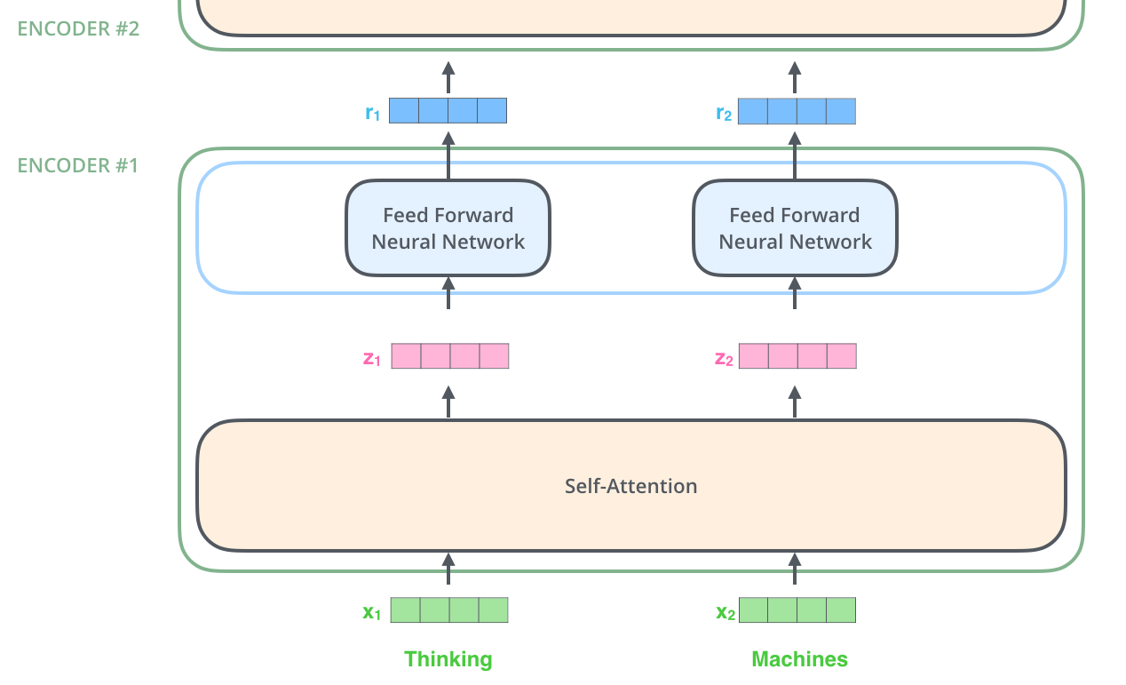
The first step in calculating self-attention is to create three vectors from each of the encoder’s input vectors (in this case, the embedding of each word). So for each word, we create a Query vector, a Key vector, and a Value vector. These vectors are created by multiplying the embedding by three matrices that we trained during the training process.
计算自注意力的第一步就是从每个编码器的输入向量(每个单词的词向量)中生成三个向量。也就是说对于每个单词,我们创造一个查询向量、一个键向量和一个值向量。这三个向量是通过词嵌入与三个权重矩阵后相乘创建的。
Notice that these new vectors are smaller in dimension than the embedding vector. Their dimensionality is 64, while the embedding and encoder input/output vectors have dimensionality of 512. They don’t HAVE to be smaller, this is an architecture choice to make the computation of multiheaded attention (mostly) constant.
可以发现这些新向量在维度上比词嵌入向量更低。他们的维度是64,而词嵌入和编码器的输入/输出向量的维度是512. 但实际上不强求维度更小,这只是一种基于架构上的选择,它可以使多头注意力(multiheaded attention)的大部分计算保持不变。
![]()
Multiplying x1 by the WQ weight matrix produces q1, the "query" vector associated with that word. We end up creating a "query", a "key", and a "value" projection of each word in the input sentence.
X1与WQ权重矩阵相乘得到q1, 就是与这个单词相关的查询向量。最终使得输入序列的每个单词的创建一个查询向量、一个键向量和一个值向量。
What are the “query”, “key”, and “value” vectors?
什么是查询向量、键向量和值向量向量?
They’re abstractions that are useful for calculating and thinking about attention. Once you proceed with reading how attention is calculated below, you’ll know pretty much all you need to know about the role each of these vectors plays.
它们都是有助于计算和理解注意力机制的抽象概念。请继续阅读下文的内容,你就会知道每个向量在计算注意力机制中到底扮演什么样的角色。
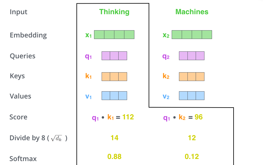
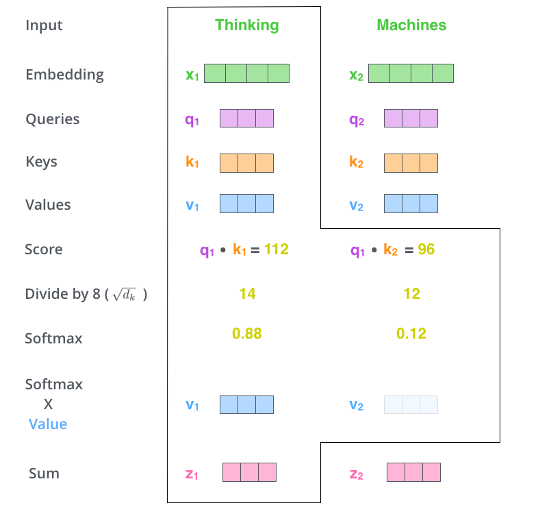
The second step in calculating self-attention is to calculate a score. Say we’re calculating the self-attention for the first word in this example, “Thinking”. We need to score each word of the input sentence against this word. The score determines how much focus to place on other parts of the input sentence as we encode a word at a certain position.
计算自注意力的第二步是计算得分。假设我们在为这个例子中的第一个词“Thinking”计算自注意力向量,我们需要计算输入句子中的每个单词与“Thinking”之间的关系分(dependency score)。这些分数决定了在编码单词“Thinking”的过程中需要多少其他单词的参与。
The score is calculated by taking the dot product of the query vector with the key vector of the respective word we’re scoring. So if we’re processing the self-attention for the word in position #1, the first score would be the dot product of q1 and k1. The second score would be the dot product of q1 and k2.
这些分数是通过打分单词(所有输入句子的单词)的键向量与“Thinking”的查询向量相点积来计算的。所以如果我们是处理位置最靠前的词的自注意力的话,第一个分数是q1和k1的点积,第二个分数是q1和k2的点积。
![]()
The third and forth steps are to divide the scores by 8 (the square root of the dimension of the key vectors used in the paper – 64. This leads to having more stable gradients. There could be other possible values here, but this is the default), then pass the result through a softmax operation. Softmax normalizes the scores so they’re all positive and add up to 1.
第三步和第四步是将分数除以8(8是论文中使用的键向量的维数64的平方根,这会让梯度更稳定。这里也可以使用其它值,8只是默认值),然后通过softmax传递结果。softmax的作用是使所有单词的分数归一化,得到的分数都是正值且和为1。
This softmax score determines how much how much each word will be expressed at this position. Clearly the word at this position will have the highest softmax score, but sometimes it’s useful to attend to another word that is relevant to the current word.
这个softmax分数决定了每个单词对编码当下位置(“Thinking”)的贡献(注:按照我的理解就是其他单词与当前待编码单词的相关程度)。显然,已经在这个位置上的单词将获得最高的softmax分数,但有时关注另一个与当前单词相关的单词也会有帮助。
The fifth step is to multiply each value vector by the softmax score (in preparation to sum them up). The intuition here is to keep intact the values of the word(s) we want to focus on, and drown-out irrelevant words (by multiplying them by tiny numbers like 0.001, for example).
第五步是将每个值向量乘以softmax分数(这是为了准备之后将它们求和)。这里的直觉是希望关注语义上相关的单词,并弱化不相关的单词(例如,让它们乘以0.001这样的小数)。
The sixth step is to sum up the weighted value vectors. This produces the output of the self-attention layer at this position (for the first word).
第六步是对加权值向量求和(译注:自注意力的另一种解释就是在编码某个单词时,就是将所有单词的表示(值向量)进行加权求和,而权重是通过该词的id(键向量)与被编码词请求(查询向量)的点积并通过softmax得到。),然后即得到自注意力层在该位置的输出(在我们的例子中是对于第一个单词)。
That concludes the self-attention calculation. The resulting vector is one we can send along to the feed-forward neural network. In the actual implementation, however, this calculation is done in matrix form for faster processing. So let’s look at that now that we’ve seen the intuition of the calculation on the word level.
这样自自注意力的计算就完成了。得到的向量就可以独立传给前馈神经网络。然而实际中,这些计算是以矩阵形式完成的,以便算得更快。那我们接下来就看看如何用矩阵实现的。
Matrix Calculation of Self-Attention
The first step is to calculate the Query, Key, and Value matrices. We do that by packing our embeddings into a matrix X, and multiplying it by the weight matrices we’ve trained (WQ, WK, WV).
第一步是计算查询矩阵、键矩阵和值矩阵。为此,我们将将输入句子的词嵌入装进矩阵X中,将其乘以我们训练的权重矩阵(WQ,WK,WV)。
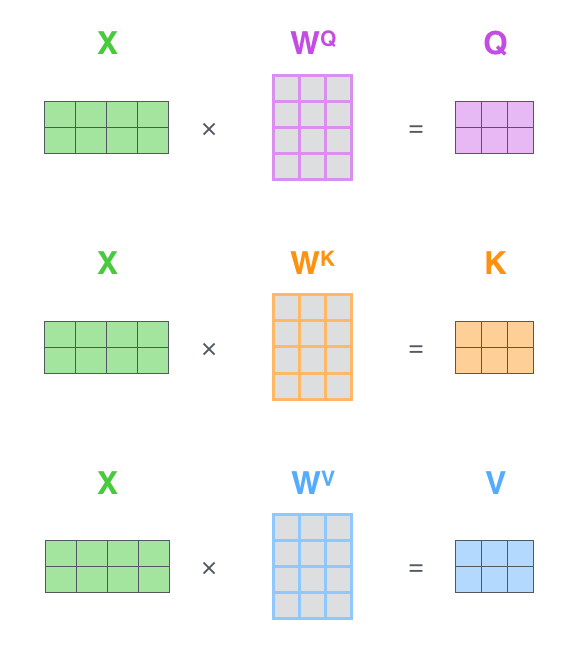
Every row in the X matrix corresponds to a word in the input sentence. We again see the difference in size of the embedding vector (512, or 4 boxes in the figure), and the q/k/v vectors (64, or 3 boxes in the figure)
x矩阵中的每一行对应于输入句子中的一个单词。我们再次看到词嵌入向量 (512,或图中的4个格子)和q/k/v向量(64,或图中的3个格子)的大小差异。
Finally, since we’re dealing with matrices, we can condense steps two through six in one formula to calculate the outputs of the self-attention layer.
最后,由于我们处理的是矩阵,我们可以将步骤2到步骤6合并为一个公式来计算自注意力层的输出。
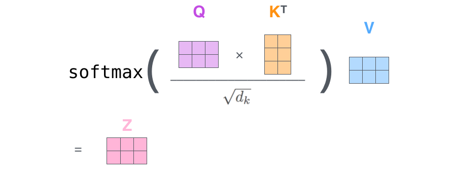
The self-attention calculation in matrix form