第三十一周学习笔记

Facial Keypoint Detection

项目学习自这里

实验名：人脸关键点(Facial keypoints，也称为facial landmarks)检测
实验目的：训练一个卷积神经网络，以检测图片上人脸的关键点
数据集：YouTube Faces Dataset
pipline:

加载并可视化数据集，共计5770张彩色图片，3462张训练，2308张测试，图片名和关键点位置信息在一个csv文件中，每行是一张图片，按如下方式组织

第1列	第2列到第137列
图片名	每两列是一个点

创建数据集类进行图像变换
Batching并加载数据
构建网络，并测试网络的参数是否fit（通过输入样例，比较输出与期望输出的维度）
写出网络在测试样例运行的函数，以及可视化测试结果的函数，排除网络的参数错误
训练
测试

实验结论
1.本次实验我首先尝试了CS231n中介绍的几个简单的网络，比如简单的INPUT->CONV->RELU->POOL->FC，以及INPUT->[CONV->RELU->POOL]*2->FC等结构，结果发现，训练误差根本无法下降，说明这些网络的表达能力很低，且在设置网络参数时，如何设置输出channel是一个十分头疼的问题，于是考虑了resnet18
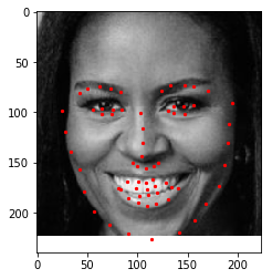
2.实验选择resnet18作为网络结构，首先以MSE作为损失函数，选择优化方法为Adam，得到的结果在测试集的表现如下
在这里插入图片描述
3.选择损失函数为smoothl1loss，结果如下
l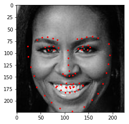

由结果可见，脸部的scale对结果还是有很大的影响，同时smoothl1loss的训练结果优于MSE，在实际训练中，MSE训练到35轮左右在测试集上的误差便不再下降，而smoothl1loss训练到46轮左右仍然继续下降。

本次实验还表明了resnet有很好的图片信息提取能力，即便在原架构上几乎不做任何改动（除输入和输出外）直接套用，仍然可以达到如此的效果，其次误差的选择也很重要，适合问题的误差会更容易优化
some codes：
1.从pandas中读取数据集

image_name = key_pts_frame.iloc[n, 0]
key_pts = key_pts_frame.iloc[n, 1:].as_matrix()
key_pts = key_pts.astype('float').reshape(-1,2)

2.显示数据集的代码，采用的是matplotlib，将点和图片同时进行展示

import matplotlib.pyplot as plt
import matplotlib.image as mpimg
import os

def show_keypoints(image, key_pts):
	""""show image with keypoints"""
	plt.imshow(image)
	plt.scatter(key_pts[:,0],key_pts[:,1],s=10,maker='.',c='r')

plt.figure(figsize=(5,5))
show_keypoints(mpimg.imread(os.path.join('data/',image_name)),key_pts)
plt.show()

3.数据集类
参考自PyTorch data loading tutorial
注意，其中的skimage被换成了matplotlib中的图片io方法

torch.utils.data.Dataset是一个数据集的抽象类，这个类可以让我们加载批数据集，并在我们的数据集上进行同样的变换，比如缩放和正则化图片

自定义的数据集必须继承Dataset并重写以下方法：

__len__，使得len(dataset)返回数据集的大小
__getitem__，来支持索引dataset[i]，从而得到第i个数据

这里使用了一个技巧，在数据集类的__init__方法中只读csv文件而不读图片文件，在真正需要返回图片的_getitem__文件中才读取文件，从而节省内存

from torch.utils.data imprt Dataset, DataLoader
class FacialKeypoinntsDataset(Dataset):
	"""Face Landmarks Dataset."""
	
	def __init__(self, csv_file, wftiroot_dir, transform=None):
		"""
		Args:
			csv_file (string): Path to the csv file with annotations.
			root_dir (string): Directory with all the images.
			transform (callable, optional): Optional transform to be applied on a sample
		"""
		self.key_pts_frame = pd.read_csv(csv_file)
		self.root_dir = root_dir
		self.traansform = transform
	def __len__(self):
		return len(self.key_pts_frame)

	def __getitem(self, idx):
		image_name = os.path.join(self.root_dir,
		self.key_pts_frame.iloc[idx,0])
		image = npimge.imread(image_name)

		# if image has an alpha color channrl, get rid of it
		if (image.shape[2] == 4):
			image = image[:,:,0:3]
		
		key_pts = self.key_ts_frame.iloc[idx, 1:].as_matrix()
		key_pts = key_pts.astype('float').reshape(-1,2)
		sample = {'image':image, 'keypoints':key_pts}

		if self.transform:
			sample = self.transform(sample)
		
		return sample

4.变换
神经网络需要同样大小的图片进行输入，并且颜色和坐标需要经过标准化，且Pytorch需要将numpy变为Tensors作为输入，因此需要以下四个方法：

Normalize:将彩色图片转化为[0,1]中的灰度图，且将关键点标准化到[-1,1]中
Rescale：将图片缩放到期望的大小
RandomCrop：随机裁剪图片
ToTensor:将图片转化为torch中的图片

变换的写法采用的是写一个callable的类

import torch
from torchvision import transforms, utils
# tranforms

class Normalize(object):
    """Convert a color image to grayscale and normalize the color range to [0,1]."""        

    def __call__(self, sample):
        image, key_pts = sample['image'], sample['keypoints']
        
        image_copy = np.copy(image)
        key_pts_copy = np.copy(key_pts)

        # convert image to grayscale
        image_copy = cv2.cvtColor(image, cv2.COLOR_RGB2GRAY)
        
        # scale color range from [0, 255] to [0, 1]
        image_copy=  image_copy/255.0
        
        # scale keypoints to be centered around 0 with a range of [-1, 1]
        # mean = 100, sqrt = 50, so, pts should be (pts - 100)/50
        key_pts_copy = (key_pts_copy - 100)/50.0


        return {'image': image_copy, 'keypoints': key_pts_copy}


class Rescale(object):
    """Rescale the image in a sample to a given size.

    Args:
        output_size (tuple or int): Desired output size. If tuple, output is
            matched to output_size. If int, smaller of image edges is matched
            to output_size keeping aspect ratio the same.
    """

    def __init__(self, output_size):
        assert isinstance(output_size, (int, tuple))
        self.output_size = output_size

    def __call__(self, sample):
        image, key_pts = sample['image'], sample['keypoints']

        h, w = image.shape[:2]
        if isinstance(self.output_size, int):
            if h > w:
                new_h, new_w = self.output_size * h / w, self.output_size
            else:
                new_h, new_w = self.output_size, self.output_size * w / h
        else:
            new_h, new_w = self.output_size

        new_h, new_w = int(new_h), int(new_w)

        img = cv2.resize(image, (new_w, new_h))
        
        # scale the pts, too
        key_pts = key_pts * [new_w / w, new_h / h]

        return {'image': img, 'keypoints': key_pts}


class RandomCrop(object):
    """Crop randomly the image in a sample.

    Args:
        output_size (tuple or int): Desired output size. If int, square crop
            is made.
    """

    def __init__(self, output_size):
        assert isinstance(output_size, (int, tuple))
        if isinstance(output_size, int):
            self.output_size = (output_size, output_size)
        else:
            assert len(output_size) == 2
            self.output_size = output_size

    def __call__(self, sample):
        image, key_pts = sample['image'], sample['keypoints']

        h, w = image.shape[:2]
        new_h, new_w = self.output_size

        top = np.random.randint(0, h - new_h)
        left = np.random.randint(0, w - new_w)

        image = image[top: top + new_h,
                      left: left + new_w]

        key_pts = key_pts - [left, top]

        return {'image': image, 'keypoints': key_pts}


class ToTensor(object):
    """Convert ndarrays in sample to Tensors."""

    def __call__(self, sample):
        image, key_pts = sample['image'], sample['keypoints']
         
        # if image has no grayscale color channel, add one
        if(len(image.shape) == 2):
            # add that third color dim
            image = image.reshape(image.shape[0], image.shape[1], 1)
            
        # swap color axis because
        # numpy image: H x W x C
        # torch image: C X H X W
        image = image.transpose((2, 0, 1))
        
        return {'image': torch.from_numpy(image),
                'keypoints': torch.from_numpy(key_pts)}

data_transform = transforms.Compose([Rescale(250),
                                     RandomCrop(224),
                                     Normalize(),
                                     ToTensor()])
                                     
transformed_dataset = FacialKeypointsDataset(csv_file='data/training_frames_keypoints.csv',
                                             root_dir='data/training/',
                                             transform=data_transform)

要注意变换的顺序，先rescale再crop，从而不会出现因原始图片尺寸不同而crop大小不一定适用所有图片的问题
5.批量化并加载数据

batch_size = 10
train_loader = DataLoader(transformed_dataset,
						batch_size=batch_size,
						shuffle=True, # 打乱
						num_workers=4) # num of subprocess

6.神经网络
一个网络的示例

import torch.nn as nn
import torch.nn.functional as F


class Net(nn.Module):
    def __init__(self):
        super(Net, self).__init__()
        self.conv1 = nn.Conv2d(3, 6, 5)
        self.pool = nn.MaxPool2d(2, 2)
        self.conv2 = nn.Conv2d(6, 16, 5)
        self.fc1 = nn.Linear(16 * 5 * 5, 120)
        self.fc2 = nn.Linear(120, 84)
        self.fc3 = nn.Linear(84, 10)

    def forward(self, x):
        x = self.pool(F.relu(self.conv1(x)))
        x = self.pool(F.relu(self.conv2(x)))
        x = x.view(-1, 16 * 5 * 5)
        x = F.relu(self.fc1(x))
        x = F.relu(self.fc2(x))
        x = self.fc3(x)
        return x


net = Net()
import torch.optim as optim

criterion = nn.CrossEntropyLoss()
optimizer = optim.SGD(net.parameters(), lr=0.001, momentum=0.9)

7.flatten层

class Flatten(nn.Module):
    def forward(self, x):
        return x.view(x.shape[0], -1)

注意事项

图片需要经过变换，使得大小相同
numpy和pytorch记录图片的方式不一样，numpy image: H x W x C，torch image: C X H X W，所以要通过image = image.transpose((2, 0, 1))来将tensor中的图片
本任务不是一个分类任务，所以选择损失函数时应该选择适合回归任务的损失函数，比如MSE或L1/SmoothL1，具体在这里

CS231n

激活函数

翻译自英文笔记

Sigmoid

$\sigma(x)=1/(1+e^{-x})$

在这里插入图片描述
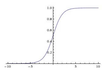
sigmoid将数字压缩到0到1之间，sigmoid函数本身能够很好地解释为神经元的激发率（概率），但实践中，sigmoid函数很少被使用了，因为

sigmoid函数饱和导致的梯度消失：当sigmoid激活在0或者1的位置时，梯度几乎接近于0，在反向传播时，这个梯度需要和别的值相乘，因此，这会导致梯度消失的问题，而且，我们要十分关注权值初始化的问题来避免饱和，如果权值初始化过大，则网络饱和，因而很难进行学习
sigmoid的输出不是以0为中心的：这导致后一层的神经元输入不是以0为中心，根据公式 $f=w^Tx+b$ ，则 $w$ 的梯度非正即负，使得梯度下降出现锯齿现象（类似最速下降的感觉，两次梯度更新的方向接近垂直，导致权值更新过慢）。不过一个batch的梯度add up之后往往会解决这个问题，因此这个问题并不像之前的问题一样严重

Tanh

$tanh(x)=2\sigma(2x)-1$

在这里插入图片描述
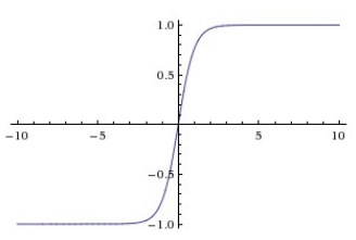
tanh将输入压缩到[-1,1]中，与sigmoid相同，它会出现饱和，但它的输出是以0为中心的，因此实践中相比sigmoid人们更倾向选择tanh，实际上tanh是一个缩放了的sigmoid，如上面的公式所示

Relu

$relu(x)=max(x,0)$

在这里插入图片描述

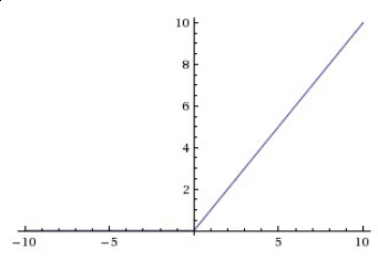
线性整流单元（Rectified Linear Unit）最近十分热门，它有以下的优缺点：

(+)相比使用sigmoid和tanh，它加速了神经网络的收敛速度，这是因为它的线性非饱和特性
(+)相比使用sigmoid和tanh，计算更简单，消耗的计算资源更小
(-)可能会"die"，举个例子，一个大的梯度通过ReLU可能会导致这个ReLU单元再也不在任何数据上激活，从而之后的梯度会永远是0，这样的单元就类似于die的状态

Leaky ReLU

$f(x)=1(x<0)(\alpha x)+1(x>=0)(x)$
Leaky ReLU是一个对于dying ReLU问题的补救，相比与对小于0的输入不予激活，leaky ReLU会有一个小的slope，上式中 $\alpha$ 是一个小的常数。

Maxout

$f(x)=max(w_1^Tx+b_1,w_2^Tx+b_2)$ ，这是由Goodfellow等人引入的，注意到ReLU和leaky ReLU是它的特例，它享有ReLU单元的所有优点，但它使得每个神经元的参数多了两倍，也消耗了更多的计算资源。

应该使用什么激活神经元呢

首先使用ReLU，注意学习率的大小避免"dead"，也可以试试Leaky ReLU或Maxout，永远别用sigmoid，可以试试tanh但应该期望它比ReLU/Maxout表现差

网络层数的选择

深层的网络更容易过拟合，但我们不通过选择浅层的网络来避免过拟合，实践中，通过一些之后介绍的避免过拟合的方法来控制过拟合。

其中的深层的原因是，浅层的网络难以使用局部的方法（例如梯度下降）来训练，因为浅层的网络有更少的局部极小值点，虽然更容易逼近，但这些极小值点表现差异太大，需要通过随机初始化和一些运气才能找到好的网络，而大的网络极小值点多，但这些极小值点的表现都差异不大（且通常比小的网络表现好），因此更容易训练

绝对不要因为害怕过拟合而使用小的网络，而是使用大的网络，再通过一些特殊的方法来避免过拟合

翻译自英文笔记

预处理

常见的预处理错误：值得一提的是所有预处理统计量（比如数据均值）都应该从训练集中计算，然后应用到验证和测试集上，例如，在所有数据上计算均值，并减去均值，再分为训练、验证、测试集是错误的做法，应该在训练集上计算得到均值，然后在验证和测试集上减去才是正确的做法

权值初始化

陷阱：0初始化，将所有权值都初始化为0会导致网络各个神经元对称，从而它们计算的值一样且梯度一样，在训练过程中权值的变化也一样。

小的随机数：假设权值最后是以0为中心的正态分布是合理的，但又无法将它们直接初始化为0，因此将它们初始化为小的随机数（服从正态分布或均匀分布，两者表现差不多）

注意：并非初始值越小越好，如果初始值太小，会导致梯度消失的问题

统一方差：
直接使用小的随机数初始化会导致输出的方差因为输入的维度不同而不同
$Var(s)=(nVar(w))Var(x)$
具体证明需要用到这个
因此我们可以通过w=np.random.randn(n)/sqrt(n)来初始化，从而统一方差

其他的类似idea的初始化方法有

$Var(w)=2/(n_{in}+n_{out})$
$Var(w)=2/n$ ，这是实践中比较推荐用于ReLU神经元的初始化方法

**稀疏初始化：**将所有权重矩阵设为0，为了打破对称性，每个神经元都与下一层固定的神经元随机连接（有一个小的随机权值），这个数字通常是10

初始化偏置值：：通常被初始化为0，使用ReLU时，被设定为0.01以便开始的时候神经元可以激活，但尚不明确这样是否能提提升性能（有时可能更差），因此通常都使用0初始化

**实践：**实践中对于使用ReLU单元的网络，通过w=np.random.randn(n)*sqrt(2.0/n)来初始化

Batch Normalization：
实践中Batch Normalization对初始化更有鲁棒性，往往加在全连接或卷积层之后，非线性层之前

正则化

以下是一些避免过拟合的方法
L2正则化可能是最常见的正则化方法，它对大的权值向量进行乘法，偏向得到分散的权值向量。这样使得网络关注所有输入特征，而不会特别关注小部分特征。
L1正则化是另一种常见的正则化方法，有一种方法可以结合两种正则化方法 $\lambda_1|w|+\lambda_2w^2$ ，这叫Elastic net regularization，L1正则化方法使得权值更稀疏（也就是几乎接近0），最终提取出输入中重要的成分而与不重要的“噪声”输入无关。实践中，如果你不知道选择L1还是L2，L2应该作为首选
最大范式约束（Max norm constraints），另一种正则化方法是设定权值向量量级的上界，并使用投影梯度下降法来确保这一约束，实践中，参数先如往常一样更新，然后剔除权值以满足 $||w||_2<c$ 的条件， $c$ 一般为3或4，一些人报告说这提升了网络表现。这个方法的一个好处是当学习率太大时，它使得网络不会“爆炸”
**随机失活（Dropout）**是一个极其高效、简单的近期引入的技术。训练中，dropout以概率p（超参数）保留某个神经元，或将其设置为0
在这里插入图片描述

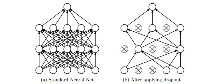
值得注意的是，dropout仅在训练过程中使用，在预测时不使用，但在预测时，我们用p scale每个神经元的激活值，因为在训练过程中它们的输出期望是p*out，为了与训练时一致，测试时也要乘上p，以下是一个不推荐的实现

""" Vanilla Dropout: Not recommended implementation (see notes below) """

p = 0.5 # probability of keeping a unit active. higher = less dropout

def train_step(X):
  """ X contains the data """
  
  # forward pass for example 3-layer neural network
  H1 = np.maximum(0, np.dot(W1, X) + b1)
  U1 = np.random.rand(*H1.shape) < p # first dropout mask
  H1 *= U1 # drop!
  H2 = np.maximum(0, np.dot(W2, H1) + b2)
  U2 = np.random.rand(*H2.shape) < p # second dropout mask
  H2 *= U2 # drop!
  out = np.dot(W3, H2) + b3
  
  # backward pass: compute gradients... (not shown)
  # perform parameter update... (not shown)
  
def predict(X):
  # ensembled forward pass
  H1 = np.maximum(0, np.dot(W1, X) + b1) * p # NOTE: scale the activations
  H2 = np.maximum(0, np.dot(W2, H1) + b2) * p # NOTE: scale the activations
  out = np.dot(W3, H2) + b3

在预测的时候我们需要乘p，但预测的表现十分重要，为此我们可以使用Inverted Dropout方法来保证预测的代码不变

""" 
Inverted Dropout: Recommended implementation example.
We drop and scale at train time and don't do anything at test time.
"""

p = 0.5 # probability of keeping a unit active. higher = less dropout

def train_step(X):
  # forward pass for example 3-layer neural network
  H1 = np.maximum(0, np.dot(W1, X) + b1)
  U1 = (np.random.rand(*H1.shape) < p) / p # first dropout mask. Notice /p!
  H1 *= U1 # drop!
  H2 = np.maximum(0, np.dot(W2, H1) + b2)
  U2 = (np.random.rand(*H2.shape) < p) / p # second dropout mask. Notice /p!
  H2 *= U2 # drop!
  out = np.dot(W3, H2) + b3
  
  # backward pass: compute gradients... (not shown)
  # perform parameter update... (not shown)


  
def predict(X):
  # ensembled forward pass
  H1 = np.maximum(0, np.dot(W1, X) + b1) # no scaling necessary
  H2 = np.maximum(0, np.dot(W2, H1) + b2)
  out = np.dot(W3, H2) + b3

偏置正则化是少用的技术，即便实际使用时并没用造成表现变差

每层正则化也是少用的技术

实践中，通常使用一个L2正则化，同时使用dropout也是常用的技术，p通常取0.5

要求

开启任务后，每周至少完成总量的25%
每个任务必须要有阶段性的目标，与总时间的目标
每四周进行一次总结，反思之前的任务进度
以后的学习笔记的开头先叙述上周目标的完成度，再写本周的笔记，最后写下周的目标
每周笔记上都要附上本要求

本周反思

本周主要完成了项目代码的学习以及cs231n笔记的继续学习，但是任务完成度仅有10%与之前规定的25%不匹配
预计cs231n的学习截止时间为第三十四周

下周目标

阅读resnet的论文
继续完成cs231n的学习进度到50%
学习opencv上册到25%