目录
综述
“明道若昧;进道若退;夷道若颣;大方无隅;大器免成;大音希声;大象无形。”
本文采用编译器:jupyter
主成分分析 是一个非监督的机器学习算法,主要作为降维方法。
先考虑这样一个问题:对于正交属性空间中的样本点,如何用一个超平面(直线的高维推广)对所有样本进行恰当的表达? 容易想到,若存在这样的超平面,那么它大概应具有这样的性质:
最近重构性:样本点到这个超平面的距离都足够近;
最大可分性:样本点在这个超平面上的投影能尽可能分开。
对于一个二维数据:
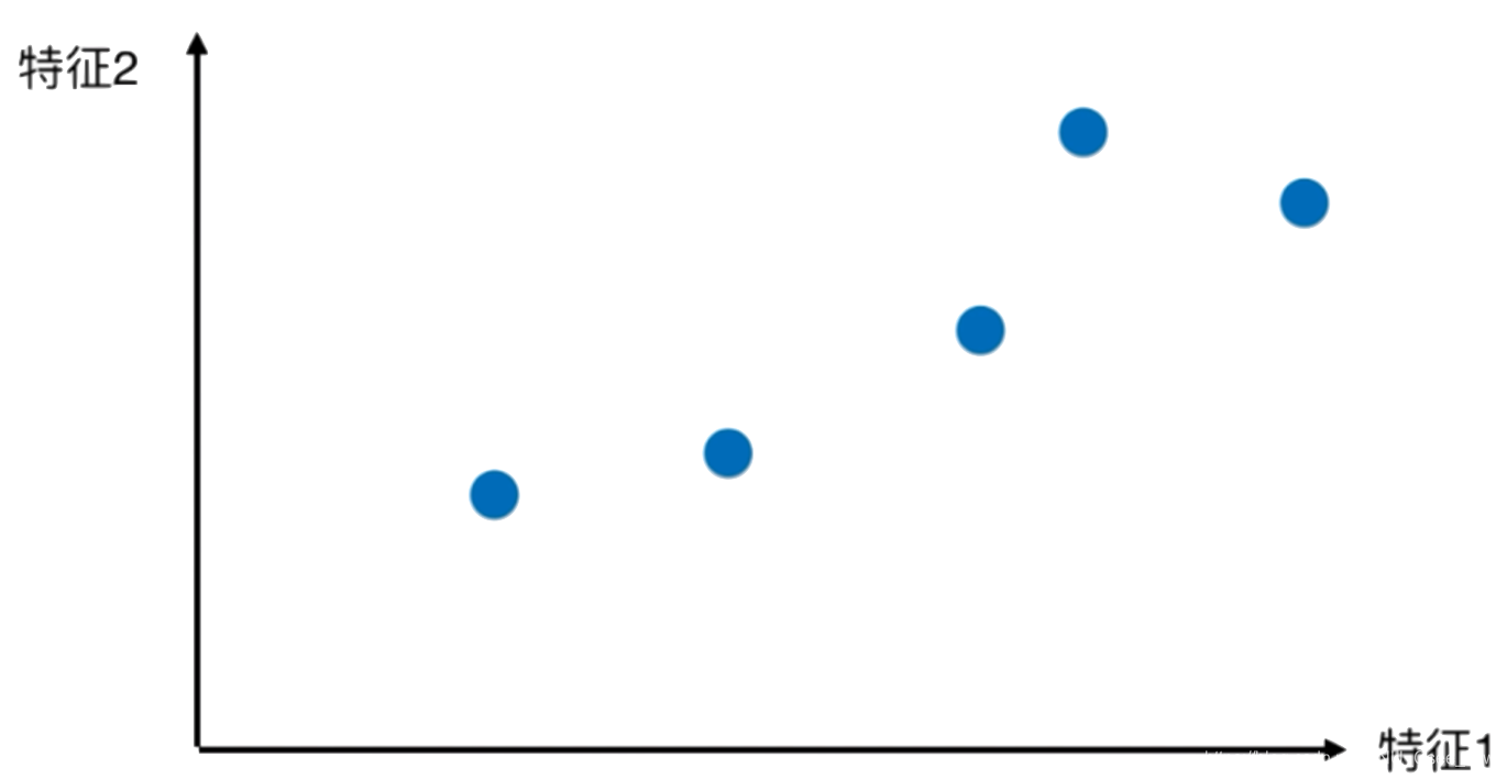
最先想到的降维方法应该是将数据全部映射到横轴或纵轴上,即只取特征1或特征2,如下图
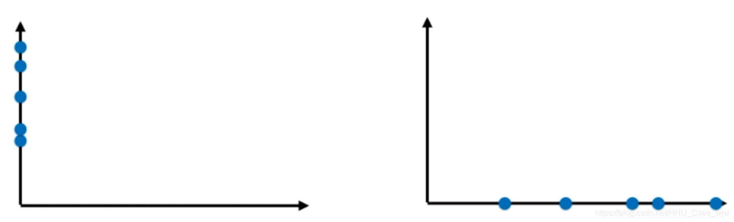
再特殊一点,将所有点映射到一条直线上,所有的点更加趋近于原来的位置
即,样本间间距最大化。
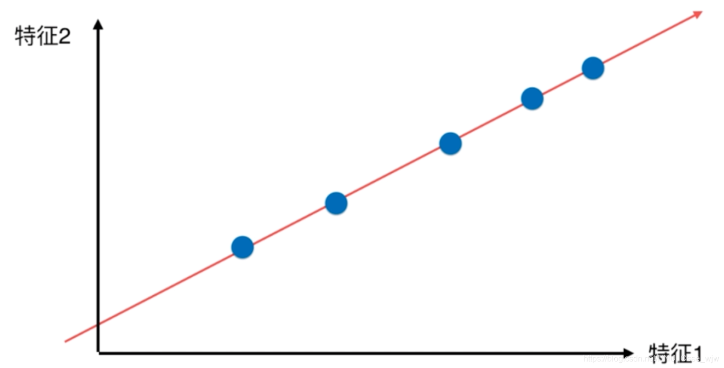
事实上,我们完全可以使用方差来描述样本间间距,方差越大,样本间间距越大。
给出简单的PCA步骤:
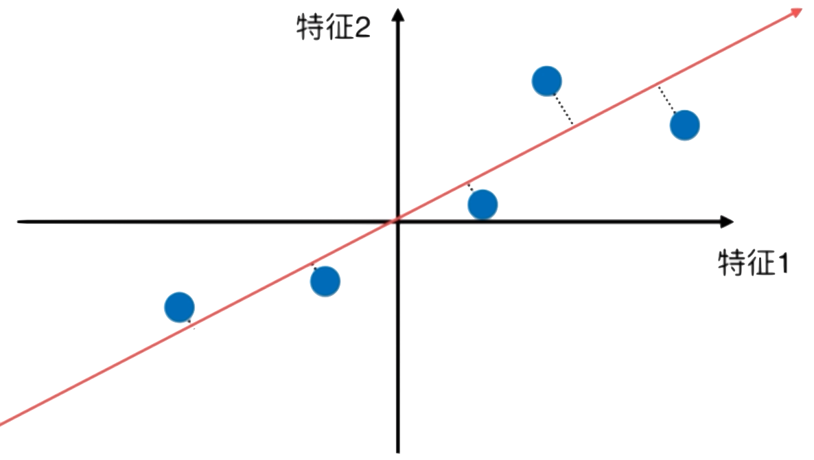
第一步:将样本的均值变为0(demean)
此时
第二步:我们想要求一个轴的方向w=(w1,w2),使得所有样本再映射到w轴之后有
最大,由向量的知识可知,一个向量点乘另一个向量的单位向量,即为在另一个向量上的投影,如下
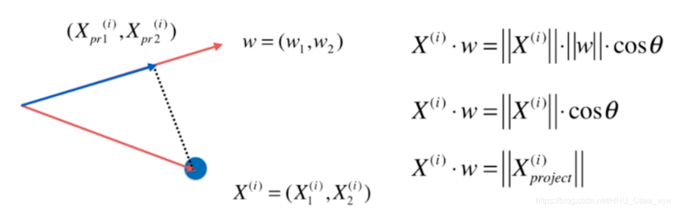
此时称为第一主成分
故最终目标表示如下:
最大
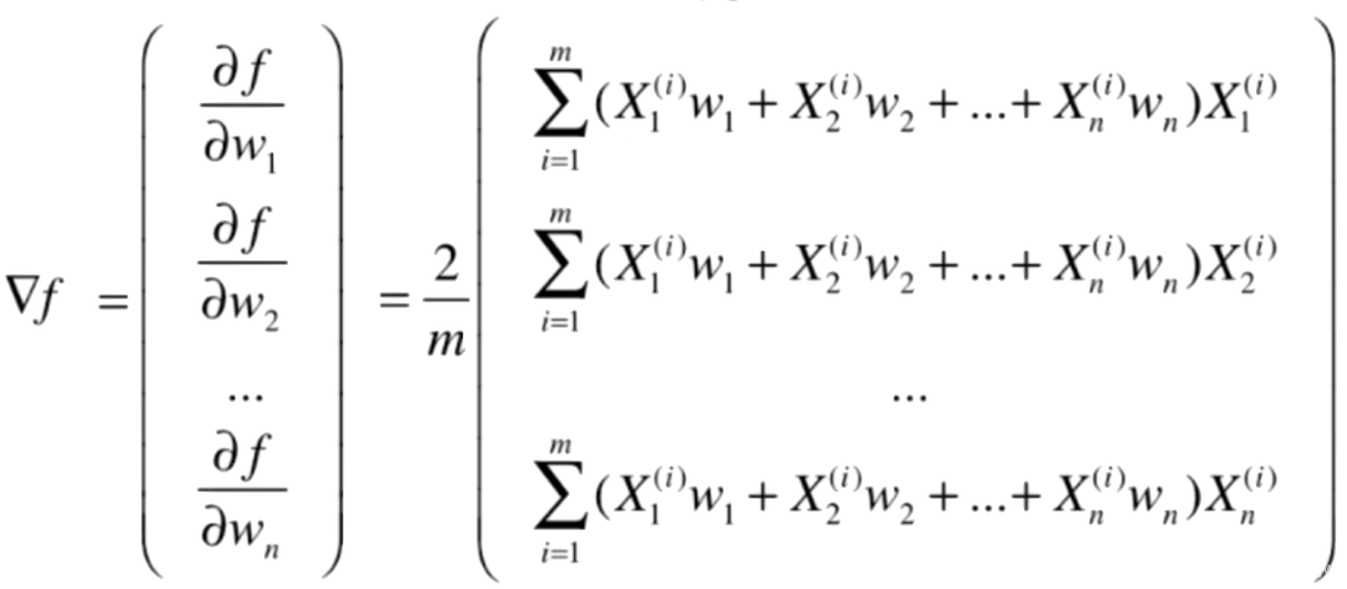
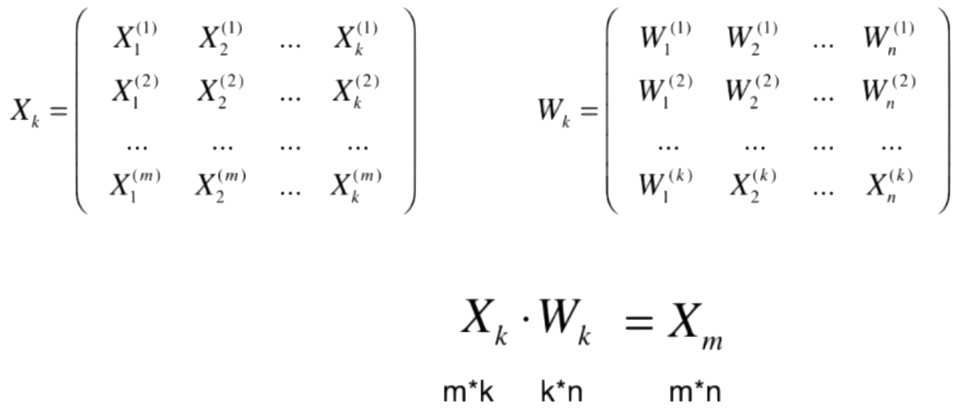
扩展到多维情况:

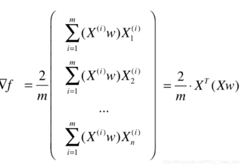
此时是一个摸表函数的最优化问题,使用梯度上升法
![]()
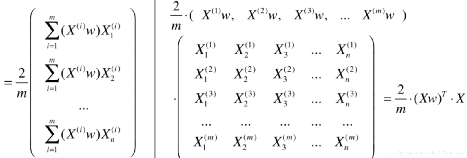
Xw是m✖️1的向量,转置后是1✖️m,X是m✖️n的向量,乘之后是1✖️n的向量,所以要对整体再进行转置,结果为
01 使用梯度上升法求解主成分
import numpy as np
import matplotlib.pyplot as plt

# 创建有两个特征,且特征之间有一定线性关系的数据
X = np.empty((100, 2))
X[:,0] = np.random.uniform(0., 100., size=100)
X[:,1] = 0.75 * X[:,0] + 3. +np.random.normal(0, 10., size=100)

plt.scatter(X[:,0], X[:,1])
plt.show()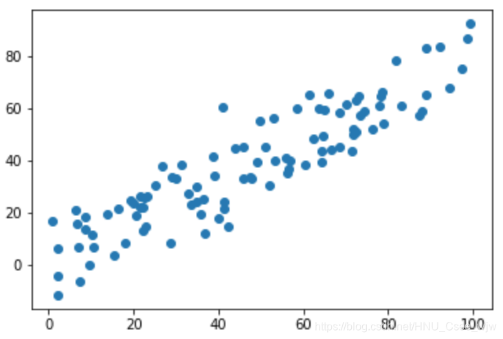
demean
# 第一步:均值归零化
def demean(X):
    return X - np.mean(X, axis=0) # 每一个样本 减去 所有样本的每一个特征的均值

X_demean = demean(X)

plt.scatter(X_demean[:,0], X_demean[:,1])
plt.show()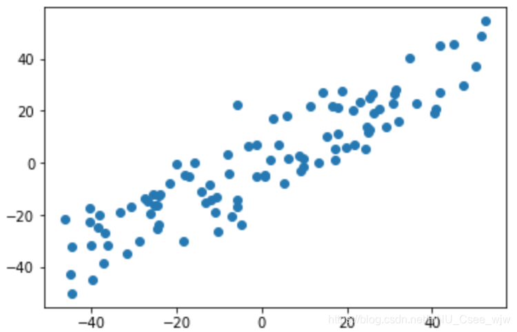
np.mean(X_demean[:,0])
# Out[7]:
# 6.1817218011128716e-15

np.mean(X_demean[:,1])
# Out[8]:
# -7.0343730840249918e-15
梯度上升法
# 目标函数,w是单位向量
def f(w, X):
return np.sum((X.dot(w) ** 2)) / len(X)
# 梯度
def df_math(w, X):
return X.T.dot(X.dot(w)) * 2. / len(X)
def df_debug(w, X, epsilon=0.0001):
res = np.empty(len(w))
for i in range(len(w)):
w_1 = w.copy()
w_1[i] += epsilon
w_2 = w.copy()
w_2[i] -= epsilon
res[i] = (f(w_1, X) - f(w_2, X)) / (2 * epsilon)
return res
# 求单位向量,向量/模
def direction(w):
return w / np.linalg.norm(w)
def gradient_ascent(df, X, initial_w, eta, n_iters = 1e4, epsilon=1e-8):
w = direction(initial_w)
cur_iter = 0
while cur_iter < n_iters:
gradient = df(w, X)
last_w = w
# 与梯度下降法不同
w = w + eta*gradient
w = direction(w)
if(abs(f(w, X) - f(last_w, X)) < epsilon):
break
cur_iter += 1
return w
initial_w = np.random.random(X.shape[1]) # 注意2:不能从0向量开始
initial_w
# Out[13]:
# array([ 0.64339125, 0.18770856])
eta = 0.001
# 注意3:不能使用StandardScaler标准化数据,因为标准化之后方差固定是1了
gradient_ascent(df_debug, X_demean, initial_w, eta)
# Out[15]:
# array([ 0.77379857, 0.63343174])
gradient_ascent(df_math, X_demean, initial_w, eta)
# Out[16]:
# array([ 0.77379857, 0.63343174])
w = gradient_ascent(df_math, X_demean, initial_w, eta)
plt.scatter(X_demean[:,0],X_demean[:,1], color='b')
plt.plot([0, w[0]*30], [0, w[1]*30], color='r')
plt.show()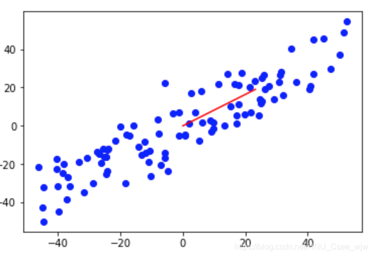
# 所求出的轴即为第一主成分

# 取一个极端情况,w的x,y方向分别是直角三角形两条边0.6与0.8
X2 = np.empty((100, 2))
X2[:,0] = np.random.uniform(0., 100., size=100)
X2[:,1] = 0.75 * X2[:,0] + 3.

plt.scatter(X2[:,0], X2[:,1])
plt.show()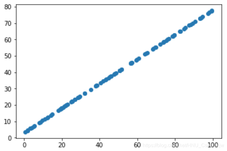
X2_demean = demean(X2)

w2 = gradient_ascent(df_math, X2_demean, initial_w, eta)

plt.scatter(X2_demean[:,0],X2_demean[:,1], color='b')
plt.plot([0, w2[0]*30], [0, w2[1]*30], color='r')
plt.show()
求出第一主成分后,如何求出下一个主成分?
答案是将数据在第一个主成分上的分量去掉,在新的数据上继续求第一主成分

02 获得前n个主成分
import numpy as np
import matplotlib.pyplot as plt
# 创建有两个特征,且特征之间有一定线性关系的数据
X = np.empty((100, 2))
X[:,0] = np.random.uniform(0., 100., size=100)
X[:,1] = 0.75 * X[:,0] + 3. +np.random.normal(0, 10., size=100)
def demean(X):
return X - np.mean(X, axis=0) # 每一个样本 减去 所有样本的每一个特征的均值
X = demean(X)
plt.scatter(X[:,0], X[:,1])
plt.show()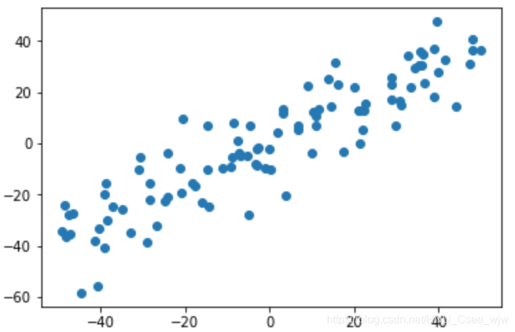
# 目标函数,w是单位向量
def f(w, X):
return np.sum((X.dot(w) ** 2)) / len(X)
# 梯度
def df(w, X):
return X.T.dot(X.dot(w)) * 2. / len(X)
# 求单位向量,向量/模
def direction(w):
return w / np.linalg.norm(w)
def first_component(X, initial_w, eta, n_iters = 1e4, epsilon=1e-8):
w = direction(initial_w)
cur_iter = 0
while cur_iter < n_iters:
gradient = df(w, X)
last_w = w
# 与梯度下降法不同
w = w + eta*gradient
w = direction(w)
if(abs(f(w, X) - f(last_w, X)) < epsilon):
break
cur_iter += 1
return w
initial_w = np.random.random(X.shape[1])
eta = 0.01
w = first_component(X, initial_w, eta)
w
# Out[8]:
# array([ 0.77652163, 0.6300906 ])
# 减去第一主成分
"""
X2 = np.empty(X.shape)
# 对每一个样本操作
for i in range (len(X)):
X2[i] = X[i] - X[i].dot(w) * w
"""
X2 = X - X.dot(w).reshape(-1, 1) * w
# X.dot(w)是一个m*1的向量,表示每一个样本在w上的模,再reshape成矩阵,最后加上方向
plt.scatter(X2[:,0], X2[:,1])
plt.show()
# 求第二主成分
w2 = first_component(X2, initial_w, eta)
w2
# Out[15]:
# array([-0.63008803,  0.77652371])

# 两个主成分相互垂直
w.dot(w2)
# Out[16]:
# 3.3080341990121553e-06

def first_n_components(n, X, eta=0.01, n_iters = 1e4, epsilon=1e-8):

    X_pca = X.copy()
    X_pca = demean(X_pca)
    res = []
    for i in range(n):
        initial_w = np.random.random(X_pca.shape[1])
        w = first_component(X_pca, initial_w, eta)
        res.append(w)

        X_pca = X_pca - X_pca.dot(w).reshape(-1, 1) * w

    return res

first_n_components(2, X)
# Out[18]:
# [array([ 0.77652176,  0.63009044]), array([-0.6300859 ,  0.77652544])]
数据恢复过程,但是由于降维操作时会丢失一部分信息,所以Xm不等于原来的X。
数据恢复实际上是在高维的空间里表示低维的数据
03 从高维数据向低维数据的映射
import numpy as np
import matplotlib.pyplot as plt
X = np.empty((100, 2))
X[:,0] = np.random.uniform(0., 100., size=100)
X[:,1] = 0.75 * X[:,0] + 3. +np.random.normal(0, 10., size=100)
from playML.PCA import PCA
pca = PCA(n_components=2)
pca.fit(X)
# Out[4]:
# PCA(n_components=2)
pca.components_
# Out[6]:
# array([[ 0.77731875, 0.62910695],
# [ 0.62911021, -0.77731612]])
pca = PCA(n_components=1)
pca.fit(X)
# Out[9]:
# PCA(n_components=1)
# 将X降维
X_reduction = pca.transform(X)
X_reduction.shape
# Out[11]:
# (100, 1)
# 将降维后的X再恢复回来
X_restore = pca.inverse_transform(X_reduction)
X_restore.shape
# Out[13]:
# (100, 2)
plt.scatter(X[:,0], X[:,1], color='b', alpha=0.5)
plt.scatter(X_restore[:,0], X_restore[:,1], color='r', alpha=0.5)
plt.show()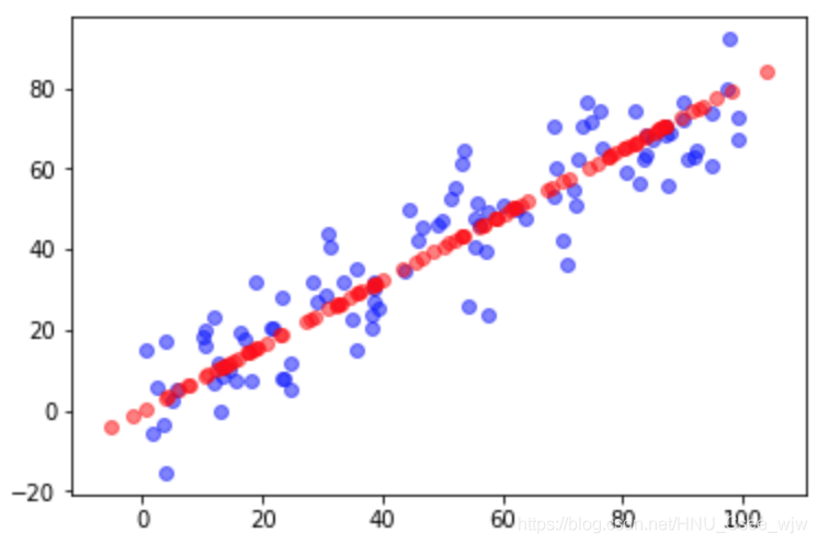
04 scikit-learn中的PCA
import numpy as np
import matplotlib.pyplot as plt
from sklearn import datasets
digits = datasets.load_digits()
X = digits.data
y = digits.target
from sklearn.model_selection import train_test_split
X_train, X_test, y_train, y_test = train_test_split(X, y, random_state=666)
X_train.shape
# Out[4]:
# (1347, 64)
%%time
from sklearn.neighbors import KNeighborsClassifier
knn_clf = KNeighborsClassifier()
knn_clf.fit(X_train, y_train)
"""
CPU times: user 16.6 ms, sys: 7.9 ms, total: 24.5 ms
Wall time: 25.7 ms
"""
knn_clf.score(X_test, y_test)
# Out[6]:
# 0.98666666666666669
# 使用PCA降维后再进行分类
from sklearn.decomposition import PCA
pca = PCA(n_components=2)
pca.fit(X_train)
X_train_reduction = pca.transform(X_train)
X_test_reduction = pca.transform(X_test)
%%time
knn_clf = KNeighborsClassifier()
knn_clf.fit(X_train_reduction, y_train)
"""
CPU times: user 2.1 ms, sys: 1.22 ms, total: 3.32 ms
Wall time: 1.91 ms
"""
knn_clf.score(X_test_reduction, y_test)
# Out[9]:
# 0.60666666666666669
# 解释方差比例,输出表示降维后两个数据维持了原来数据总方差的14%+13%
pca.explained_variance_ratio_
# Out[10]:
# array([ 0.14566817, 0.13735469])
# 先计算所有维度的方差解释比(结果从大到小排)
pca = PCA(n_components=X_train.shape[1])
pca.fit(X_train)
pca.explained_variance_ratio_
# Out[11]:
"""
array([ 1.45668166e-01, 1.37354688e-01, 1.17777287e-01,
8.49968861e-02, 5.86018996e-02, 5.11542945e-02,
4.26605279e-02, 3.60119663e-02, 3.41105814e-02,
3.05407804e-02, 2.42337671e-02, 2.28700570e-02,
1.80304649e-02, 1.79346003e-02, 1.45798298e-02,
1.42044841e-02, 1.29961033e-02, 1.26617002e-02,
1.01728635e-02, 9.09314698e-03, 8.85220461e-03,
7.73828332e-03, 7.60516219e-03, 7.11864860e-03,
6.85977267e-03, 5.76411920e-03, 5.71688020e-03,
5.08255707e-03, 4.89020776e-03, 4.34888085e-03,
3.72917505e-03, 3.57755036e-03, 3.26989470e-03,
3.14917937e-03, 3.09269839e-03, 2.87619649e-03,
2.50362666e-03, 2.25417403e-03, 2.20030857e-03,
1.98028746e-03, 1.88195578e-03, 1.52769283e-03,
1.42823692e-03, 1.38003340e-03, 1.17572392e-03,
1.07377463e-03, 9.55152460e-04, 9.00017642e-04,
5.79162563e-04, 3.82793717e-04, 2.38328586e-04,
8.40132221e-05, 5.60545588e-05, 5.48538930e-05,
1.08077650e-05, 4.01354717e-06, 1.23186515e-06,
1.05783059e-06, 6.06659094e-07, 5.86686040e-07,
7.44075955e-34, 7.44075955e-34, 7.44075955e-34,
7.15189459e-34])
"""
# 计算前i个方差解释比的和
plt.plot([i for i in range(X_train.shape[1])],
[np.sum(pca.explained_variance_ratio_[:i+1]) for i in range(X_train.shape[1])])
plt.show()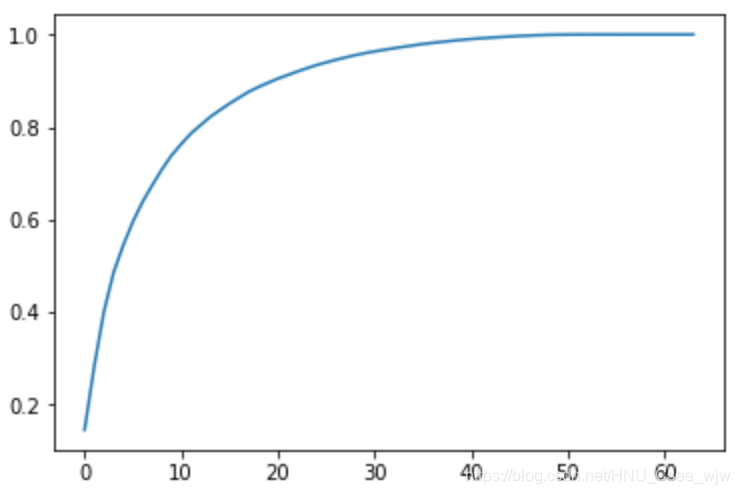
pca = PCA(0.95) # 设定主成分个数可以解释95%的方差
pca.fit(X_train)
# Out[13]:
"""
PCA(copy=True, iterated_power='auto', n_components=0.95, random_state=None,
  svd_solver='auto', tol=0.0, whiten=False)
"""

pca.n_components_
# Out[14]:
# 28

X_train_reduction = pca.transform(X_train)
X_test_reduction = pca.transform(X_test)

%%time
knn_clf = KNeighborsClassifier()
knn_clf.fit(X_train_reduction, y_train)
CPU times: user 2.38 ms, sys: 1.02 ms, total: 3.4 ms
Wall time: 2.55 ms

knn_clf.score(X_test_reduction, y_test)
# Out[17]:
# 0.97999999999999998

# 降维到2维的意义是可以进行可视化
pca = PCA(n_components=2)
pca.fit(X_train)
X_reduction = pca.transform(X)

X_reduction.shape
# Out[19]:
# (1797, 2)

for i in range(10):
    plt.scatter(X_reduction[y==i, 0], X_reduction[y==i, 1], alpha=0.8)
plt.show()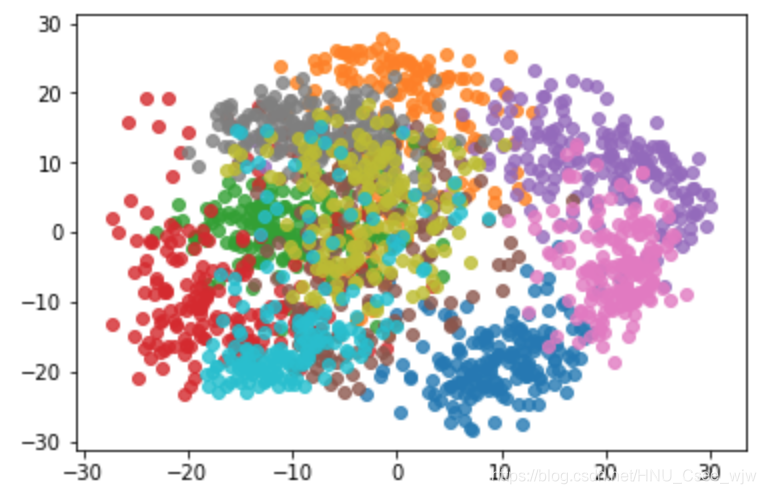
# 观察图像可知,在二维条件下橙色与蓝色,粉色等完全可分
05 使用PCA降噪
回忆之前的例子,下面两个图展示的是PCA可以用来降噪的效果
import numpy as np
import matplotlib.pyplot as plt

X = np.empty((100, 2))
X[:,0] = np.random.uniform(0., 100., size=100)
X[:,1] = 0.75 * X[:,0] + 3. + np.random.normal(0, 5, size=100)

plt.scatter(X[:,0], X[:,1])
plt.show()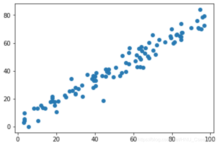
from sklearn.decomposition import PCA
pca = PCA(n_components=1)
pca.fit(X)
X_reduction = pca.transform(X)
X_restore = pca.inverse_transform(X_reduction)
plt.scatter(X_restore[:,0], X_restore[:,1])
plt.show()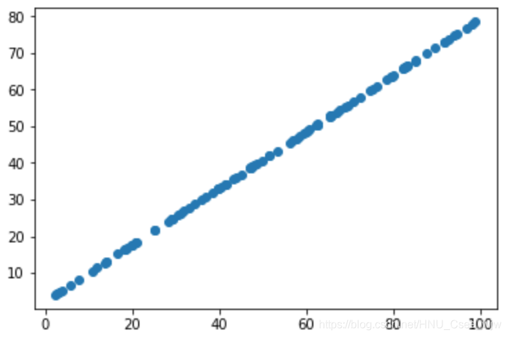
手写识别例子
from sklearn import datasets
digits = datasets.load_digits()
X = digits.data
y = digits.target
noisy_digits = X + np.random.normal(0, 4, size=X.shape)
# 从y=0中的数据中取前10个
example_digits = noisy_digits[y==0,:][:10]
for num in range(1, 10):
X_num = noisy_digits[y==num,:][:10]
example_digits = np.vstack([example_digits, X_num])
# 0-9这十个数字,每个数字10个数据
example_digits.shape
# Out[17]:
# (100, 64)
def plot_digits(data):
fig, axes = plt.subplots(10, 10, figsize=(10, 10),
subplot_kw={'xticks':[], 'yticks':[]},
gridspec_kw = dict(hspace=0.1, wspace=0.1))
for i,ax in enumerate(axes.flat):
ax.imshow(data[i].reshape(8,8),
cmap='binary', interpolation='nearest',
clim=(0, 16))
plt.show()
plot_digits(example_digits)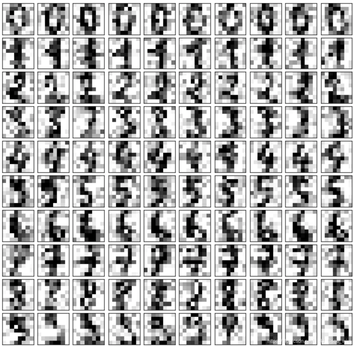
# 使用PCA进行降噪
pca = PCA(0.5)
pca.fit(noisy_digits)
# Out[22]:
"""
PCA(copy=True, iterated_power='auto', n_components=0.5, random_state=None,
  svd_solver='auto', tol=0.0, whiten=False)
"""

pca.n_components_
# Out[23]:
# 12

components = pca.transform(example_digits)
filtered_digits = pca.inverse_transform(components)
plot_digits(filtered_digits)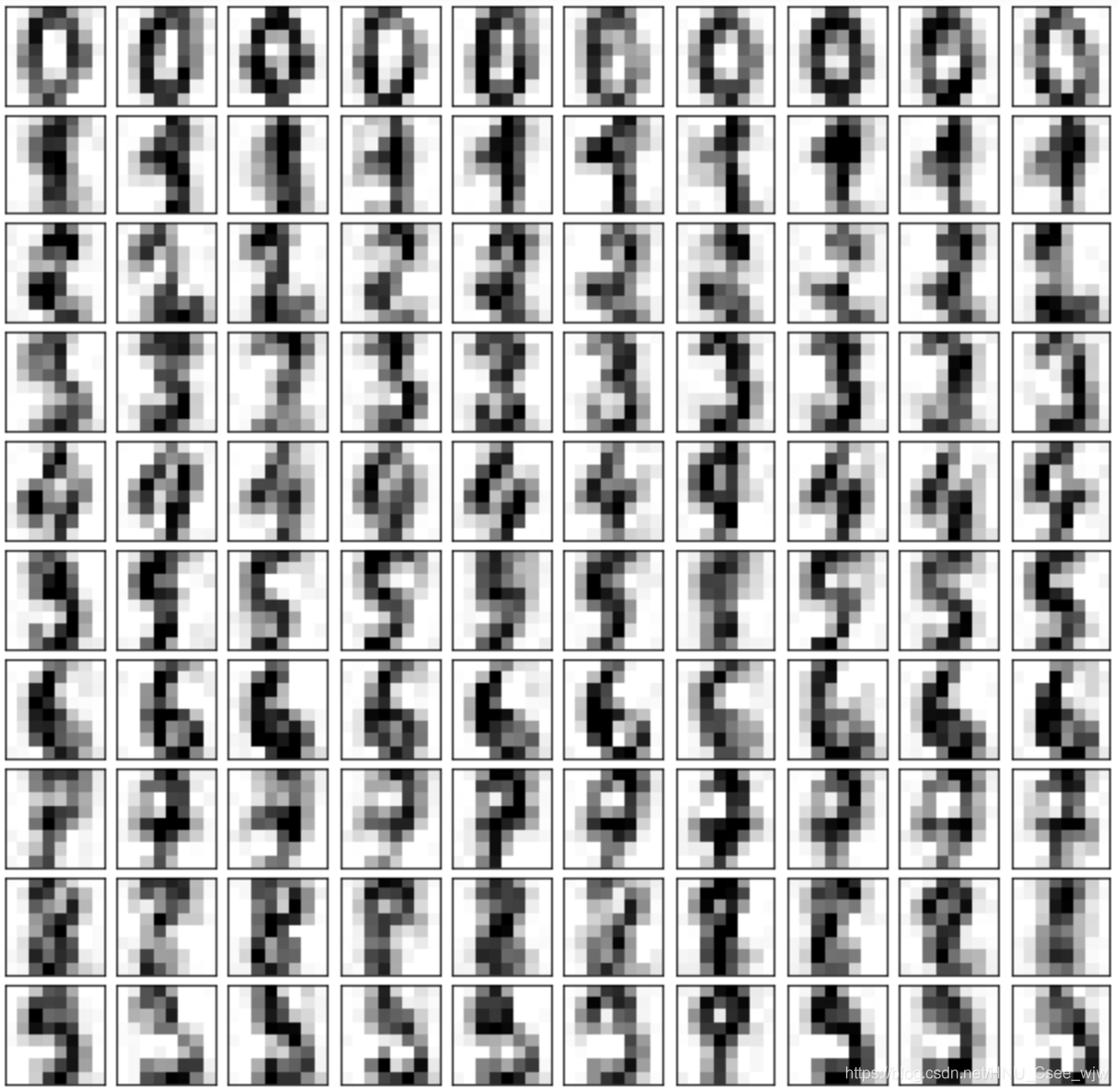
人脸识别

在人脸识别时,X的每一行可以看成一个人脸,而W的每一行则是一个特征脸,每一个特征脸实际上是人脸的一个成分
06 特征脸
import numpy as np
import matplotlib.pyplot as plt
from sklearn.datasets import fetch_lfw_people
faces = fetch_lfw_people()
faces.keys()
# Out[6]:
# dict_keys(['data', 'images', 'target', 'target_names', 'DESCR'])
faces.data.shape
# Out[7]:
# (13233, 2914)
# 图像像素
faces.images.shape
# Out[8]:
# (13233, 62, 47)
random_indexes = np.random.permutation(len(faces.data))
X = faces.data[random_indexes]
# 取随机的36张脸
example_faces = X[:36,:]
example_faces.shape
# Out[10]:
# (36, 2914)
def plot_faces(faces):
fig, axes = plt.subplots(6, 6, figsize=(10, 10),
subplot_kw={'xticks':[], 'yticks':[]},
gridspec_kw=dict(hspace=0.1, wspace=0.1))
for i,ax in enumerate(axes.flat):
ax.imshow(faces[i].reshape(62,47), cmap='bone')
plt.show()
plot_faces(example_faces)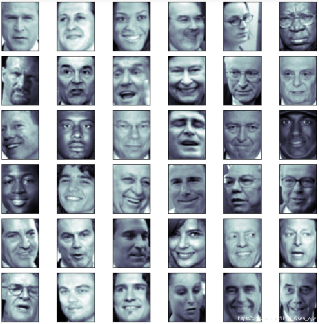
faces.target_names
# Out[14]:
"""
array(['AJ Cook', 'AJ Lamas', 'Aaron Eckhart', ..., 'Zumrati Juma',
       'Zurab Tsereteli', 'Zydrunas Ilgauskas'],
      dtype='<U35')
"""

len(faces.target_names)
# Out[15]:
# 5749
特征脸
%%time
from sklearn.decomposition import PCA
pca = PCA(svd_solver='randomized') # 使用随机方式求PCA,速度快一点
pca.fit(X)
"""
CPU times: user 2min, sys: 2.57 s, total: 2min 3s
Wall time: 56.1 s
"""

pca.components_.shape # 共2914个主成分,每个主成分对应2914个特征向量
# Out[19]:
# (2914, 2914)

plot_faces(pca.components_) # 绘制特征脸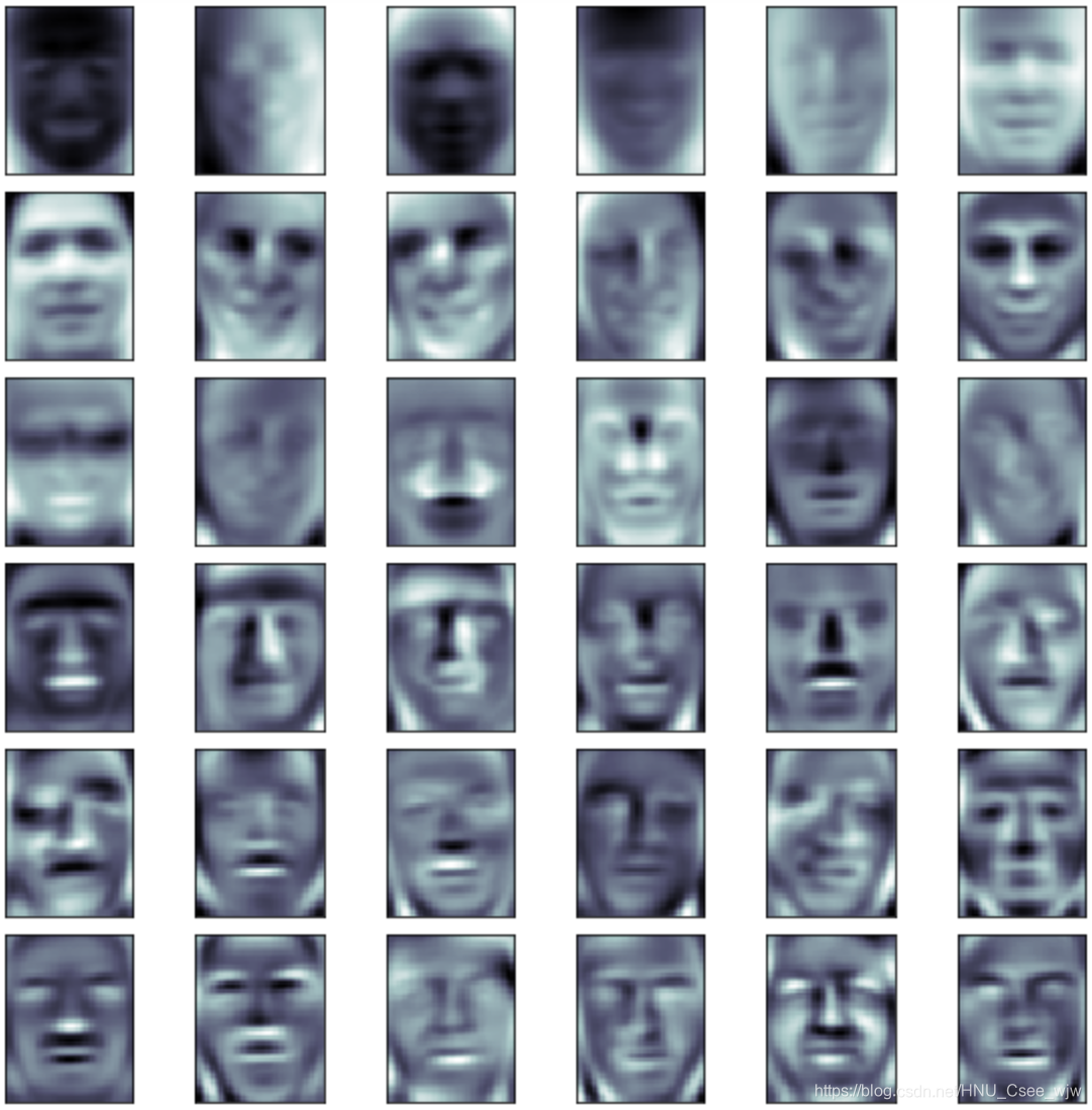
# 只取至少有60张照片的人脸
faces2 = fetch_lfw_people(min_faces_per_person=60)

faces2.data.shape
# Out[23]:
# (1348, 2914)

faces2.target_names
# Out[24]:
"""
array(['Ariel Sharon', 'Colin Powell', 'Donald Rumsfeld', 'George W Bush',
       'Gerhard Schroeder', 'Hugo Chavez', 'Junichiro Koizumi',
       'Tony Blair'],
      dtype='<U17')
"""

# 共8个人,每个人至少60张照片
len(faces2.target_names)
# Out[25]:
# 8
剩下的就可以随便玩人脸数据集啦ing。。。。
附件:
pca.py
import numpy as np


class PCA:

    def __init__(self, n_components):
        """初始化PCA"""
        assert n_components >= 1, "n_components must be valid"
        self.n_components = n_components
        self.components_ = None # 储存n_components个主成分

    def fit(self, X, eta=0.01, n_iters=1e4):
        """获得数据集X的前n个主成分"""
        # 降维后的维数应该比降维前小
        assert self.n_components <= X.shape[1], \
            "n_components must not be greater than the feature number of X"

        def demean(X):
            return X - np.mean(X, axis=0)

        def f(w, X):
            return np.sum((X.dot(w) ** 2)) / len(X)

        # 梯度
        def df(w, X):
            return X.T.dot(X.dot(w)) * 2. / len(X)

        # 求单位向量,向量/模
        def direction(w):
            return w / np.linalg.norm(w)

        def first_component(X, initial_w, eta, n_iters=1e4, epsilon=1e-8):

            w = direction(initial_w)
            cur_iter = 0

            while cur_iter < n_iters:
                gradient = df(w, X)
                last_w = w

                # 与梯度下降法不同
                w = w + eta * gradient
                w = direction(w)

                if (abs(f(w, X) - f(last_w, X)) < epsilon):
                    break

                cur_iter += 1

            return w

        X_pca = demean(X)
        self.components_ = np.empty(shape=(self.n_components, X.shape[1]))
        for i in range(self.n_components):
            initial_w = np.random.random(X_pca.shape[1])
            w = first_component(X_pca, initial_w, eta, n_iters)
            self.components_[i,:] = w

            X_pca = X_pca - X_pca.dot(w).reshape(-1, 1) * w

        return self

    def transform(self, X):
        """将给定的X,映射到各个主成分分量中"""
        assert X.shape[1] == self.components_.shape[1]

        return X.dot(self.components_.T)

    def inverse_transform(self, X):
        """将给定的X,反向映射回原来的特征空间"""
        assert X.shape[1] == self.components_.shape[0]

        return X.dot(self.components_)

    def __repr__(self):
        return "PCA(n_components=%d)" % self.n_components
最后,欢迎各位读者共同交流,祝好。
