综述
“看二更云,三更月,四更天。”
本文采用编译器:jupyter
给定训练样本集D,分类学习最基本的想法就是基于训练集D的样本空间中找到一个划分超平面,将不同类别的样本分开。但能将训练样本分开但划分超平面可能有很多,如图。
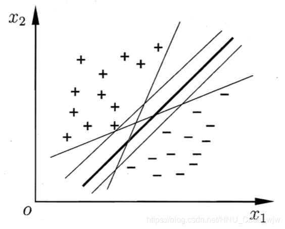
直观上看,应该去找位于两类训练样本"正中间"的划分超平面,即图中粗线的那个,因为该划分超平面对训练样本局部扰动的"容忍性"最好。例如,由于训练集的局限性或噪声的因素,训练集外的样本可能比图 中的训练 样本更接近两个类的分隔界,这将使许多划分超平面出现错误,而粗线的超平面受影响最小.换言之,这个划分超平面所产生的分类结果是最鲁棒的,对未见示例的泛化能力最强。
定义支持向量:距离分解平面最近且距离为d的向量。
在实际使用SVM时,因为涉及距离,所以要做数据标准化处理。

margin = 2d,SVM要最大化d
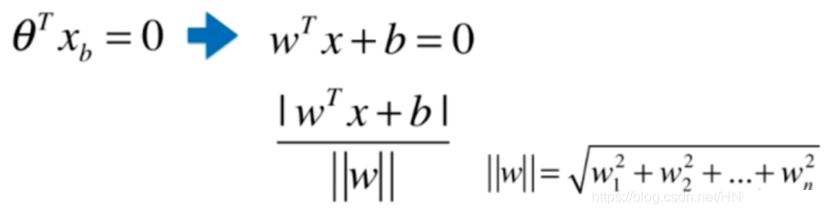
回忆解析几何中,点到直线距离为:
拓展到n维空间中:
根据支持向量机的定义,有:
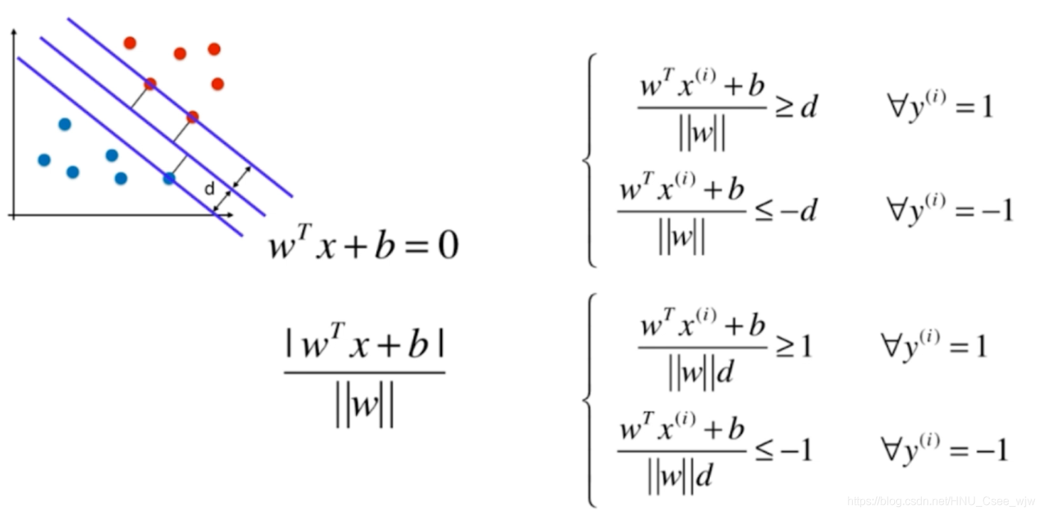
继续化简如下:
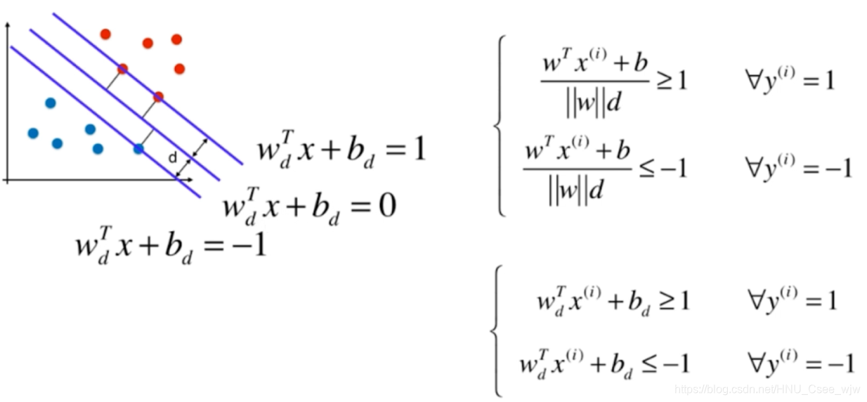
将复杂的变量名重新命名:

对于任意支持向量x,我们有目标,通常取
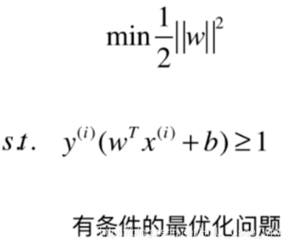
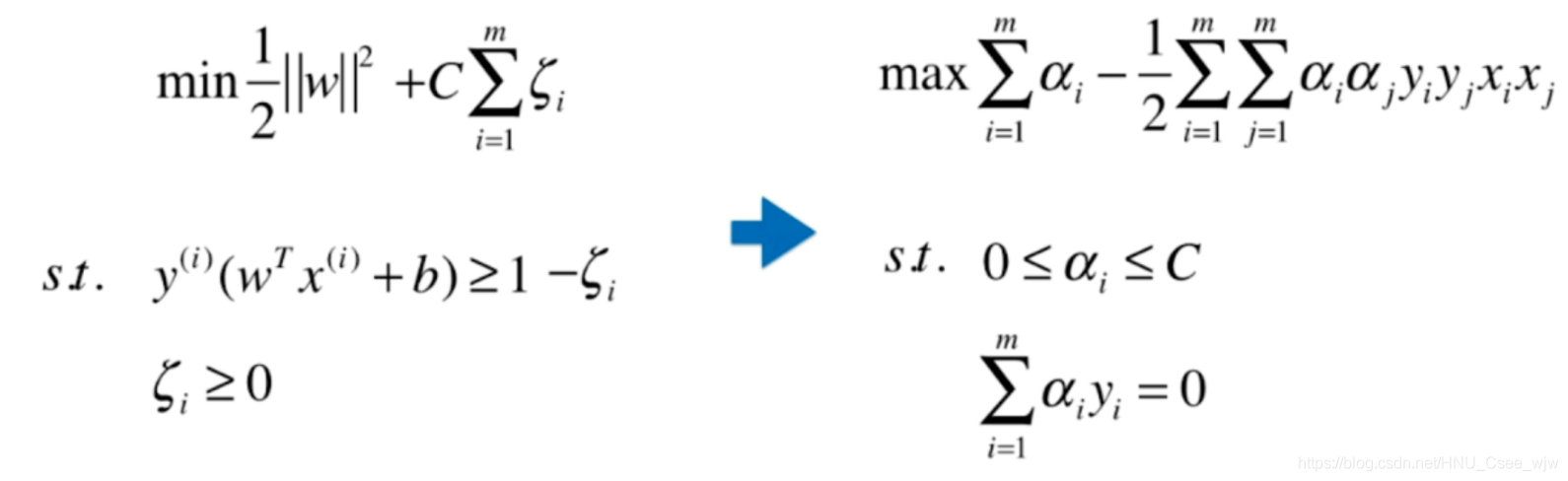
所以SVM求解的数学表达式如下:
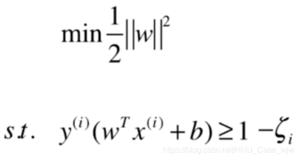
至此,我们介绍的都是硬决策边界,即要求所有的特征点都在margin范围之外,但实际上为了防止特殊的点影响模型的良好泛化能力,允许将一些点进行错误的分类。

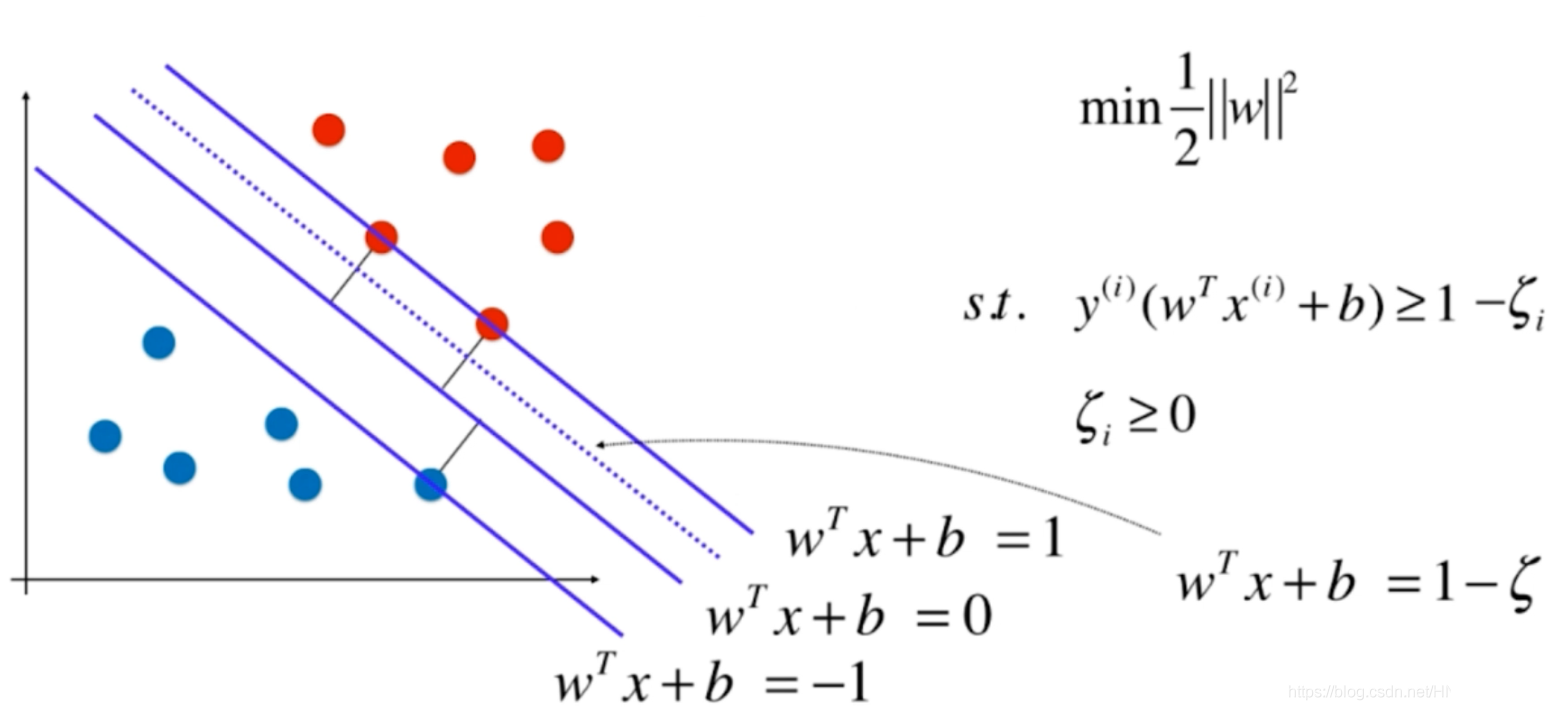
设置可以容忍的程度参数
意义如图:
为了防止容忍参数过大,应当适当的添加正则项
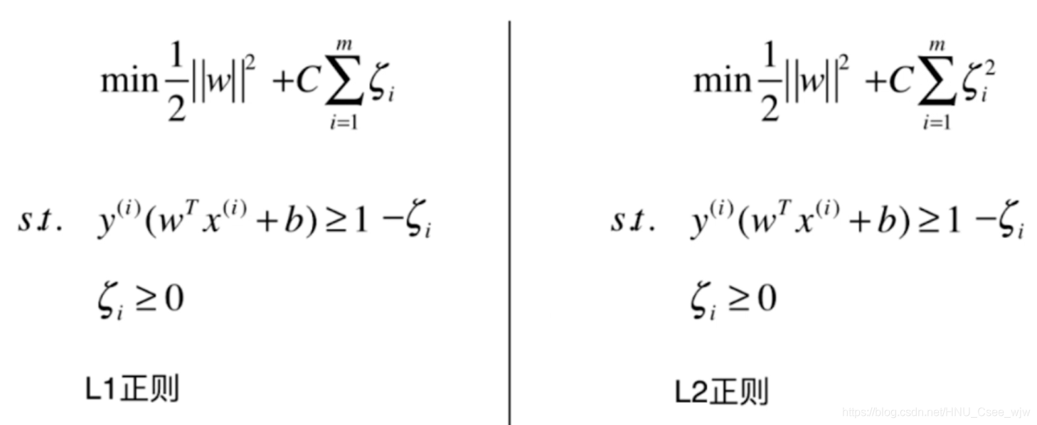
C取值越大,模型越趋近于hard margin SVM,C取值越小,模型的容错空间越大。
01 scikit-learn中的SVM
import numpy as np
import matplotlib.pyplot as plt
from sklearn import datasets
iris = datasets.load_iris()
X = iris.data
y = iris.target
X = X[y<2,:2]
y = y[y<2]
plt.scatter(X[y==0,0], X[y==0,1], color='red')
plt.scatter(X[y==1,0], X[y==1,1], color='blue')
plt.show()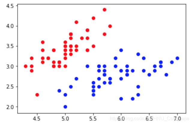
from sklearn.preprocessing import StandardScaler
standardscaler = StandardScaler()
standardscaler.fit(X)
X_standard = standardscaler.transform(X)
from sklearn.svm import LinearSVC
# C值设置较大
svc = LinearSVC(C=1e9)
svc.fit(X_standard, y)
"""
Out[7]:
LinearSVC(C=1000000000.0, class_weight=None, dual=True, fit_intercept=True,
intercept_scaling=1, loss='squared_hinge', max_iter=1000,
multi_class='ovr', penalty='l2', random_state=None, tol=0.0001,
verbose=0)
"""
def plot_decision_boundary(model, axis):
x0, x1 = np.meshgrid(
np.linspace(axis[0], axis[1], int((axis[1]-axis[0])*100)).reshape(-1,1),
np.linspace(axis[2], axis[3], int((axis[3]-axis[2])*100)).reshape(-1,1)
)
X_new = np.c_[x0.ravel(), x1.ravel()]
y_predict = model.predict(X_new)
zz = y_predict.reshape(x0.shape)
from matplotlib.colors import ListedColormap
custom_cmap = ListedColormap(['#EF9A9A', '#FFF59D','#90CAF9'])
plt.contourf(x0, x1, zz, linewidth=5, cmap=custom_cmap)
plot_decision_boundary(svc, axis=[-3, 3, -3, 3])
plt.scatter(X_standard[y==0,0], X_standard[y==0,1])
plt.scatter(X_standard[y==1,0], X_standard[y==1,1])
plt.show()
# C较小,有一定容错能力
svc2 = LinearSVC(C=0.01)
svc2.fit(X_standard, y)
"""
Out[10]:
LinearSVC(C=0.01, class_weight=None, dual=True, fit_intercept=True,
     intercept_scaling=1, loss='squared_hinge', max_iter=1000,
     multi_class='ovr', penalty='l2', random_state=None, tol=0.0001,
     verbose=0)
"""

plot_decision_boundary(svc2, axis=[-3, 3, -3, 3])
plt.scatter(X_standard[y==0,0], X_standard[y==0,1])
plt.scatter(X_standard[y==1,0], X_standard[y==1,1])
plt.show()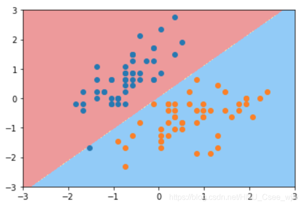
svc.coef_
# Out[12]:
# array([[ 4.03239965, -2.49294234]])

svc.intercept_
# Out[13]:
# array([ 0.95368345])

# 添加绘制margin区域的功能
def plot_svc_decision_boundary(model, axis):

    x0, x1 = np.meshgrid(
        np.linspace(axis[0], axis[1], int((axis[1]-axis[0])*100)).reshape(-1,1),
        np.linspace(axis[2], axis[3], int((axis[3]-axis[2])*100)).reshape(-1,1)
    )
    X_new = np.c_[x0.ravel(), x1.ravel()]

    y_predict = model.predict(X_new)
    zz = y_predict.reshape(x0.shape)

    from matplotlib.colors import ListedColormap
    custom_cmap = ListedColormap(['#EF9A9A', '#FFF59D','#90CAF9'])

    plt.contourf(x0, x1, zz, linewidth=5, cmap=custom_cmap)

    w = model.coef_[0]
    b = model.intercept_[0]

    # w0 * x0 + w1 * x1 + b = 0
    # => 决策边界方程 x1 = -w0/w1 * x0 - b/w1
    plot_x = np.linspace(axis[0], axis[1], 200)
    up_y = -w[0]/w[1] * plot_x - b/w[1] + 1/w[1]
    down_y = -w[0]/w[1] * plot_x - b/w[1] - 1/w[1]

    # 把取值限制在规定的y的范围内
    up_index = (up_y >= axis[2]) & (up_y <= axis[3])
    down_index = (down_y >= axis[2]) & (down_y <= axis[3])

    plt.plot(plot_x[up_index], up_y[up_index], color='black')
    plt.plot(plot_x[down_index], down_y[down_index], color='black')

plot_svc_decision_boundary(svc, axis=[-3, 3, -3, 3])
plt.scatter(X_standard[y==0,0], X_standard[y==0,1])
plt.scatter(X_standard[y==1,0], X_standard[y==1,1])
plt.show()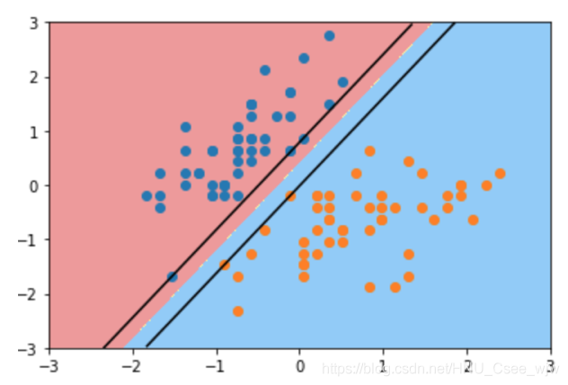
plot_svc_decision_boundary(svc2, axis=[-3, 3, -3, 3])
plt.scatter(X_standard[y==0,0], X_standard[y==0,1])
plt.scatter(X_standard[y==1,0], X_standard[y==1,1])
plt.show()
02 SVM中使用多项式特征
import numpy as np
import matplotlib.pyplot as plt
from sklearn import datasets
X, y = datasets.make_moons()
X.shape
# Out[3]:
# (100, 2)
y.shape
# Out[4]:
# (100,)
plt.scatter(X[y==0,0], X[y==0,1])
plt.scatter(X[y==1,0], X[y==1,1])
plt.show()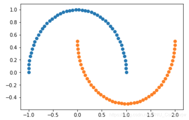
# 为数据添加噪音
X, y = datasets.make_moons(noise=0.15, random_state=666)
plt.scatter(X[y==0,0], X[y==0,1])
plt.scatter(X[y==1,0], X[y==1,1])
plt.show()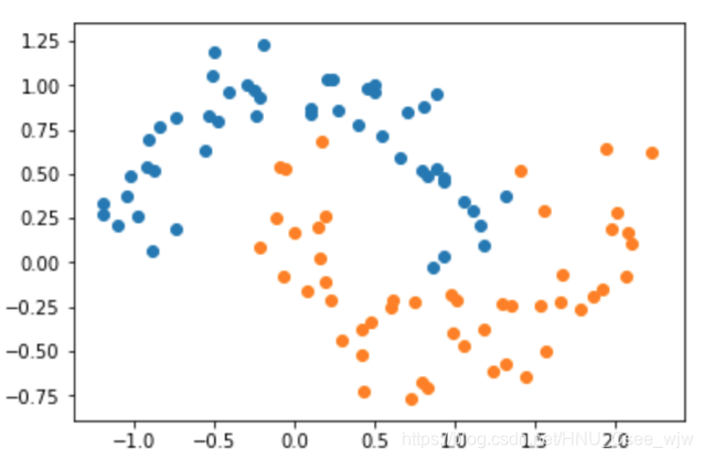
使用多项式特征的SVM
from sklearn.preprocessing import PolynomialFeatures, StandardScaler
from sklearn.svm import LinearSVC
from sklearn.pipeline import Pipeline
def PolynomialSVC(degree, C=1.0):
return Pipeline([
("poly", PolynomialFeatures(degree=degree)),
("std_scaler", StandardScaler()),
("linearSVC", LinearSVC(C=C))
])
poly_svc = PolynomialSVC(degree=3)
poly_svc.fit(X, y)
"""
Out[10]:
Pipeline(memory=None,
steps=[('poly', PolynomialFeatures(degree=3, include_bias=True, interaction_only=False)), ('std_scaler', StandardScaler(copy=True, with_mean=True, with_std=True)), ('linearSVC', LinearSVC(C=1.0, class_weight=None, dual=True, fit_intercept=True,
intercept_scaling=1, loss='squared_hinge', max_iter=1000,
multi_class='ovr', penalty='l2', random_state=None, tol=0.0001,
verbose=0))])
"""
def plot_decision_boundary(model, axis):
x0, x1 = np.meshgrid(
np.linspace(axis[0], axis[1], int((axis[1]-axis[0])*100)).reshape(-1,1),
np.linspace(axis[2], axis[3], int((axis[3]-axis[2])*100)).reshape(-1,1)
)
X_new = np.c_[x0.ravel(), x1.ravel()]
y_predict = model.predict(X_new)
zz = y_predict.reshape(x0.shape)
from matplotlib.colors import ListedColormap
custom_cmap = ListedColormap(['#EF9A9A', '#FFF59D','#90CAF9'])
plt.contourf(x0, x1, zz, linewidth=5, cmap=custom_cmap)
plot_decision_boundary(poly_svc, axis=[-1.5, 2.5, -1.0, 1.5])
plt.scatter(X[y==0,0], X[y==0,1])
plt.scatter(X[y==1,0], X[y==1,1])
plt.show()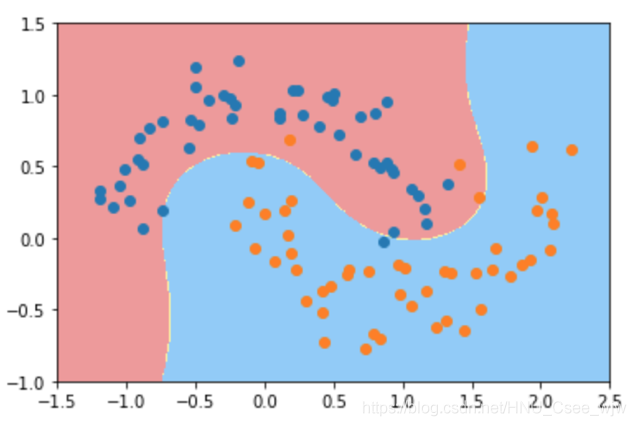
使用多项式核函数的SVM
from sklearn.svm import SVC
def PolynomialKernelSVC(degree, C=1.0):
return Pipeline([
("stad_scaler", StandardScaler()),
("kernerSVC", SVC(kernel='poly', degree=degree, C=C))
])
poly_kernel_svc = PolynomialKernelSVC(degree=3)
poly_kernel_svc.fit(X, y)
"""
Out[14]:
Pipeline(memory=None,
steps=[('stad_scaler', StandardScaler(copy=True, with_mean=True, with_std=True)), ('kernerSVC', SVC(C=1.0, cache_size=200, class_weight=None, coef0=0.0,
decision_function_shape='ovr', degree=3, gamma='auto', kernel='poly',
max_iter=-1, probability=False, random_state=None, shrinking=True,
tol=0.001, verbose=False))])
"""
plot_decision_boundary(poly_kernel_svc, axis=[-1.5, 2.5, -1.0, 1.5])
plt.scatter(X[y==0,0], X[y==0,1])
plt.scatter(X[y==1,0], X[y==1,1])
plt.show()
核函数
将SVM的表达式改写如下:
按照多项式处理办法,,
添加多项式特征后变成
,
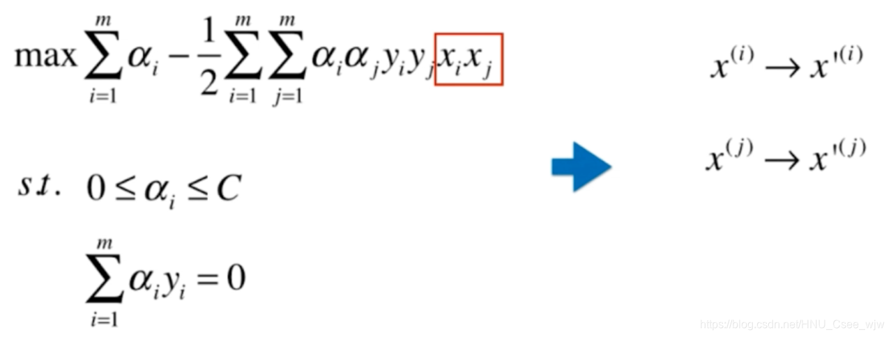
核函数的思想就是不直接添加多项式特征,而是找到一个函数K实现这种变化


y'的定义与x'相同,常数项不影响计算。如果我们直接使用核函数计算,避免先对x',y'定义,降低了计算复杂度
三种常用的核函数:K(x,y)表示x和y的点乘
多项式核函数
线性核函数
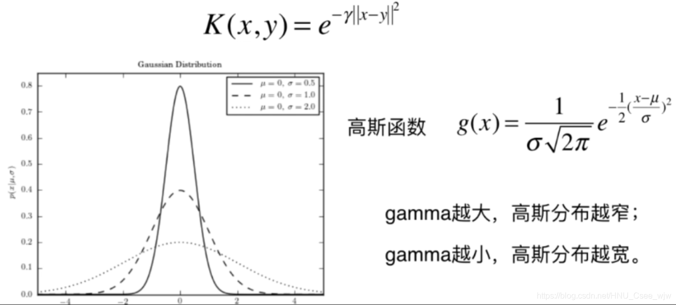
高斯核函数
高斯函数 g(x)=
有时也叫做RBF(Radial Basis Function Kernel),镜像基函数。高斯核函数的本质是将一个样本点映射到一个无穷维的特征空间,这里不做推导。
先回顾一下多项式特征:
依靠升维使得原本线性不可分的数据线性可分

原本的数据无法用一根直接来划分,我们可以添加多项式特征
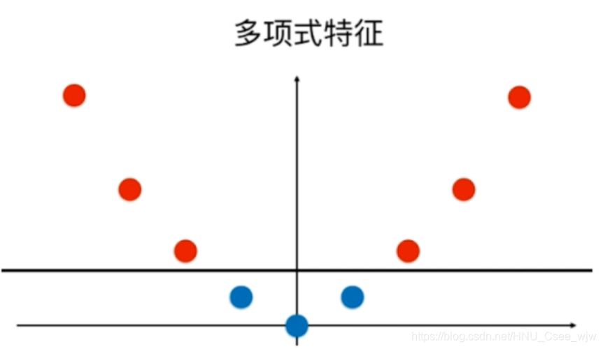
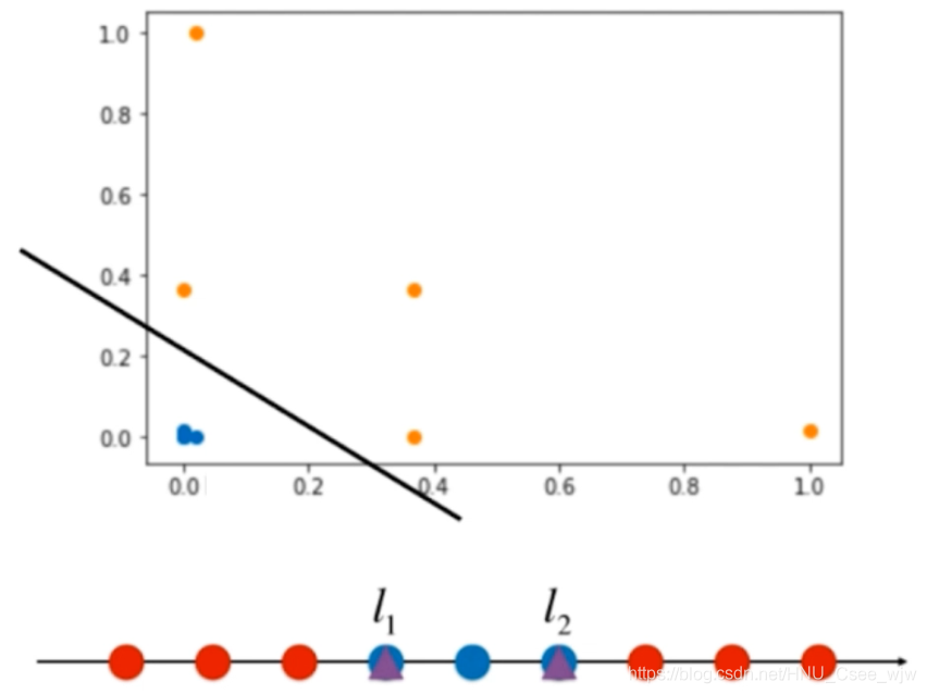
对于高斯核函数表达式中的y,如果将其作为两个固定的点l1和l2就可以得到一个二维的点,变得线性可分
![]()
高斯核:对于每一个数据点,都是landmark。m*n的数据映射成了m*m的数据。
将n维特征映射为m维特征,若果数据有m<n的特点,使用SVM就比较划算,典型的例子是自然语言处理
03 直观理解高斯核函数
import numpy as np
import matplotlib.pyplot as plt

x = np.arange(-4, 5, 1)

x
# Out[3]:
# array([-4, -3, -2, -1,  0,  1,  2,  3,  4])

# 使中间几个点的标记值为1
y = np.array((x >= -2) & (x <= 2), dtype='int')

y
# Out[5]:
# array([0, 0, 1, 1, 1, 1, 1, 0, 0])

plt.scatter(x[y==0], [0]*len(x[y==0]))
plt.scatter(x[y==1], [0]*len(x[y==1]))
plt.show()
def gaussian(x, l):
gamma = 1.0
return np.exp(-gamma * (x - l)**2)
l1, l2 = -1, 1
X_new = np.empty((len(x), 2))
for i, data in enumerate(x):
X_new[i, 0] = gaussian(data, l1)
X_new[i, 1] = gaussian(data, l2)
plt.scatter(X_new[y==0, 0], X_new[y==0, 1])
plt.scatter(X_new[y==1, 0], X_new[y==1, 1])
plt.show()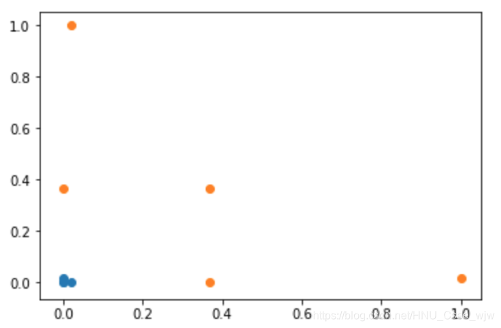
04 scikit-learn中的RBF核
import numpy as np
import matplotlib.pyplot as plt
from sklearn import datasets
X, y = datasets.make_moons(noise=0.15, random_state=666)
plt.scatter(X[y==0, 0], X[y==0, 1])
plt.scatter(X[y==1, 0], X[y==1, 1])
plt.show()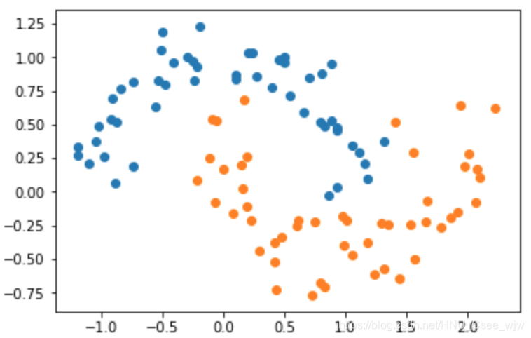
from sklearn.preprocessing import StandardScaler
from sklearn.svm import SVC
from sklearn.pipeline import Pipeline
def RBFKernelSVC(gamma=1.0):
return Pipeline([
("std_scaler", StandardScaler()),
("svc", SVC(kernel='rbf', gamma=gamma))
])
svc = RBFKernelSVC(gamma=1.0)
svc.fit(X, y)
"""
Out[4]:
Pipeline(memory=None,
steps=[('std_scaler', StandardScaler(copy=True, with_mean=True, with_std=True)), ('svc', SVC(C=1.0, cache_size=200, class_weight=None, coef0=0.0,
decision_function_shape='ovr', degree=3, gamma=1.0, kernel='rbf',
max_iter=-1, probability=False, random_state=None, shrinking=True,
tol=0.001, verbose=False))])
"""
def plot_decision_boundary(model, axis):
x0, x1 = np.meshgrid(
np.linspace(axis[0], axis[1], int((axis[1]-axis[0])*100)).reshape(-1,1),
np.linspace(axis[2], axis[3], int((axis[3]-axis[2])*100)).reshape(-1,1)
)
X_new = np.c_[x0.ravel(), x1.ravel()]
y_predict = model.predict(X_new)
zz = y_predict.reshape(x0.shape)
from matplotlib.colors import ListedColormap
custom_cmap = ListedColormap(['#EF9A9A', '#FFF59D','#90CAF9'])
plt.contourf(x0, x1, zz, linewidth=5, cmap=custom_cmap)
plot_decision_boundary(svc, axis=[-1.5, 2.5, -1.0, 1.5])
plt.scatter(X[y==0,0], X[y==0,1])
plt.scatter(X[y==1,0], X[y==1,1])
plt.show()
# gamma越大,高斯分布越窄。模型复杂度越高
svc_gamma100 = RBFKernelSVC(gamma=100)
svc_gamma100.fit(X, y)
"""
Out[7]:
Pipeline(memory=None,
     steps=[('std_scaler', StandardScaler(copy=True, with_mean=True, with_std=True)), ('svc', SVC(C=1.0, cache_size=200, class_weight=None, coef0=0.0,
  decision_function_shape='ovr', degree=3, gamma=100, kernel='rbf',
  max_iter=-1, probability=False, random_state=None, shrinking=True,
  tol=0.001, verbose=False))])
"""

plot_decision_boundary(svc_gamma100, axis=[-1.5, 2.5, -1.0, 1.5])
plt.scatter(X[y==0,0], X[y==0,1])
plt.scatter(X[y==1,0], X[y==1,1])
plt.show()
# 此时过拟合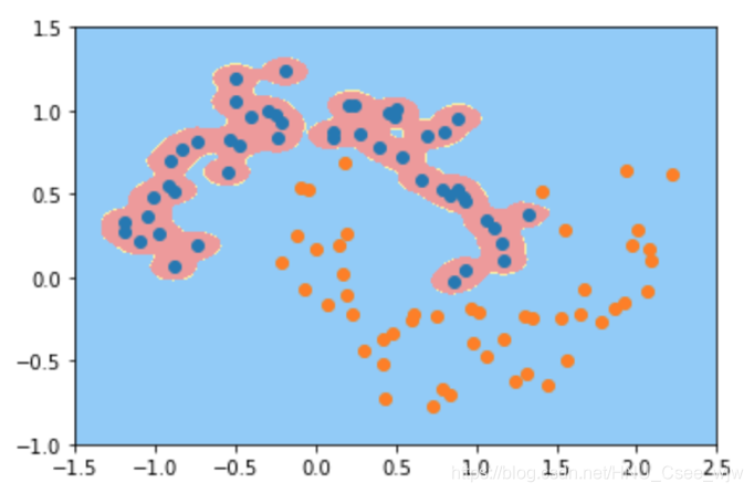
svc_gamma10 = RBFKernelSVC(gamma=10)
svc_gamma10.fit(X, y)
"""
Out[9]:
Pipeline(memory=None,
     steps=[('std_scaler', StandardScaler(copy=True, with_mean=True, with_std=True)), ('svc', SVC(C=1.0, cache_size=200, class_weight=None, coef0=0.0,
  decision_function_shape='ovr', degree=3, gamma=10, kernel='rbf',
  max_iter=-1, probability=False, random_state=None, shrinking=True,
  tol=0.001, verbose=False))])
"""

plot_decision_boundary(svc_gamma10, axis=[-1.5, 2.5, -1.0, 1.5])
plt.scatter(X[y==0,0], X[y==0,1])
plt.scatter(X[y==1,0], X[y==1,1])
plt.show()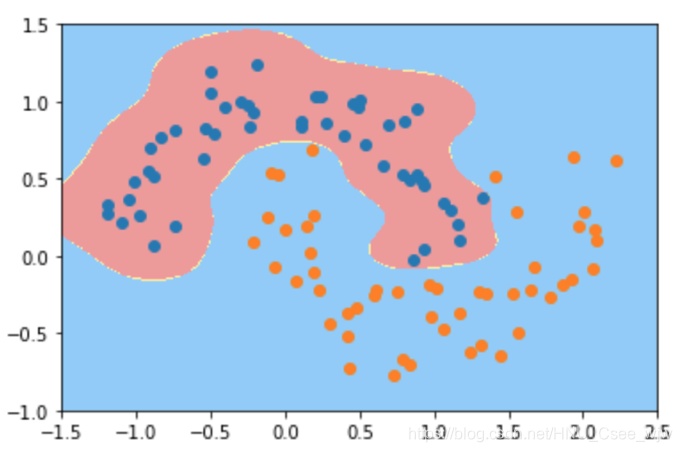
# gamma越小,高斯分布越宽。模型复杂度越低
svc_gamma05 = RBFKernelSVC(gamma=0.5)
svc_gamma05.fit(X, y)
"""
Out[11]:
Pipeline(memory=None,
     steps=[('std_scaler', StandardScaler(copy=True, with_mean=True, with_std=True)), ('svc', SVC(C=1.0, cache_size=200, class_weight=None, coef0=0.0,
  decision_function_shape='ovr', degree=3, gamma=0.5, kernel='rbf',
  max_iter=-1, probability=False, random_state=None, shrinking=True,
  tol=0.001, verbose=False))])
"""

plot_decision_boundary(svc_gamma05, axis=[-1.5, 2.5, -1.0, 1.5])
plt.scatter(X[y==0,0], X[y==0,1])
plt.scatter(X[y==1,0], X[y==1,1])
plt.show()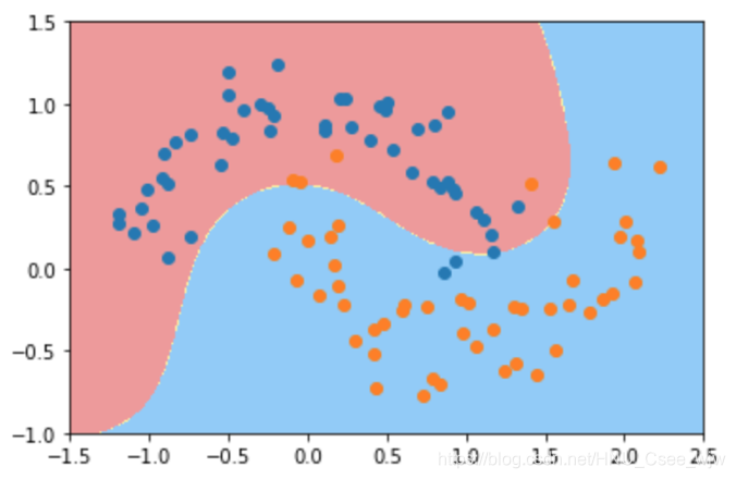
svc_gamma01 = RBFKernelSVC(gamma=0.1)
svc_gamma01.fit(X, y)
"""
Out[13]:
Pipeline(memory=None,
     steps=[('std_scaler', StandardScaler(copy=True, with_mean=True, with_std=True)), ('svc', SVC(C=1.0, cache_size=200, class_weight=None, coef0=0.0,
  decision_function_shape='ovr', degree=3, gamma=0.1, kernel='rbf',
  max_iter=-1, probability=False, random_state=None, shrinking=True,
  tol=0.001, verbose=False))])
"""

plot_decision_boundary(svc_gamma01, axis=[-1.5, 2.5, -1.0, 1.5])
plt.scatter(X[y==0,0], X[y==0,1])
plt.scatter(X[y==1,0], X[y==1,1])
plt.show()
# 此时欠拟合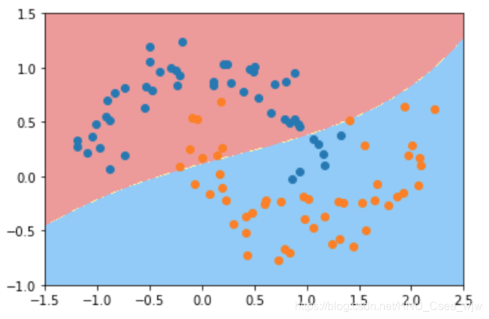
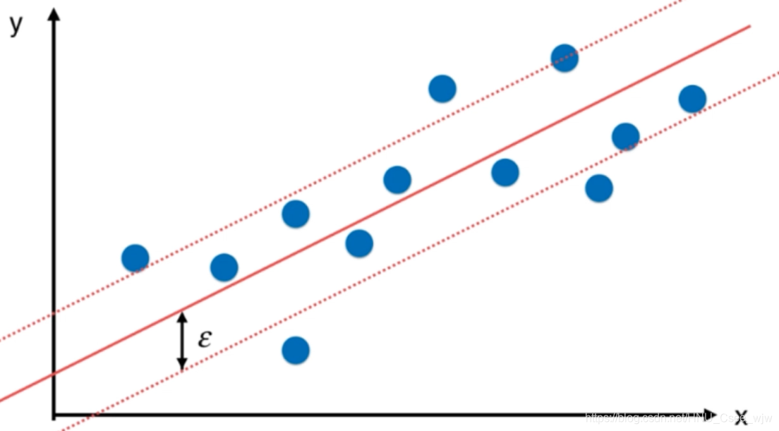
05 SVM思想解决回归问题
解决回归问题思路:使margin中间的点越多越好(和解决分类问题的思路相反),此时中间的那条线即为回归结果。
import numpy as np
import matplotlib.pyplot as plt
from sklearn import datasets
boston = datasets.load_boston()
X = boston.data
y = boston.target
from sklearn.model_selection import train_test_split
X_train, X_test, y_train, y_test = train_test_split(X, y, random_state=666)
from sklearn.svm import LinearSVR
# from sklearn.svm import SVR
from sklearn.preprocessing import StandardScaler
from sklearn.pipeline import Pipeline
def StandardLinearSVR(epsilon=0.1):
return Pipeline([
('std_scaler', StandardScaler()),
('linearSVR', LinearSVR(epsilon=epsilon))
])
svr = StandardLinearSVR()
svr.fit(X_train, y_train)
"""
Out[5]:
Pipeline(memory=None,
steps=[('std_scaler', StandardScaler(copy=True, with_mean=True, with_std=True)), ('linearSVR', LinearSVR(C=1.0, dual=True, epsilon=0.1, fit_intercept=True,
intercept_scaling=1.0, loss='epsilon_insensitive', max_iter=1000,
random_state=None, tol=0.0001, verbose=0))])
"""
svr.score(X_test, y_test)
# Out[6]:
# 0.63557199113028706最后,如果有什么疑问,欢迎和我微信交流。
