机器学习实战：信用卡欺诈行为检测

大概内容
1、解决数据不平衡的两个方式

• 下采样（Undersampling）：随机删除具有足够观察多样本的类，以便数据中类的数量比较平衡。虽然这种方法非常简单，但很有可能删除的数据中可能包含有关预测的重要信息。
• 过采样（Oversampling）：对于不平衡类（样本数少的类），随机地增加观测样本的数量，这些观测样本只是现有样本的副本，虽然增加了样本的数量，但过采样可能导致训练数据过拟合。
• 合成取样（SMOT）：该技术要求综合地制造不平衡类的样本，类似于使用最近邻分类。问题是当观察的数目是极其罕见的类时不知道怎么做。

2、标准化
3、recall衡量标准、混肴矩阵
4、模型的优化
（1）逻辑回归正则项参数的选择
（2）通过改变阈值（sigmoid）预测欺诈的可能性

现预测的数据有几十M大小，

首先读入文件，看一下文件大概内容

    data = pd.read_csv("creditcard.csv")
    data.head()

由于数据的敏感性，已将其进行PCA降维，特征用Vn代表特征，class=1，为欺诈行为

由于amount相对于其他特征量级差别很大，对其进行归一化

    from sklearn.preprocessing import StandardScaler
    
    data['normAmount'] = StandardScaler().fit_transform(data['Amount'].values.reshape(-1, 1))
    data = data.drop(['Time','Amount'],axis=1)

来看一下0/1类别的数量大小

    count_classes = pd.value_counts(data['Class'], sort = True).sort_index()
    count_classes.plot(kind = 'bar')
    plt.title("Fraud class histogram")
    plt.xlabel("Class")
    plt.ylabel("Frequency")

发现此数据有严重的不平衡问题，主要会照成一下原因：

• 由于模型/算法从来没有充分地查看全部类别信息，对于实时不平衡的类别没有得到最优化的结果；
• 由于少数样本类的观察次数极少，这会产生一个验证或测试样本的问题，即很难在类中进行表示；

1、Undersampling方法

在0类的数据中随机挑选与1数量一样的样本量，组成一组类别平衡的数据

X = data.ix[:, data.columns != 'Class']  #训练数据
y = data.ix[:, data.columns == 'Class']  #lable

#1的个数
number_records_fraud = len(data[data.Class == 1]) 
#找出1的index
fraud_indices = np.array(data[data.Class == 1].index)

# Picking the indices of the normal classes
normal_indices = data[data.Class == 0].index

#随机选出与1规模一样多的标签为0的数据（0的数据有二十多万个，1只有五百多个）
random_normal_indices = np.random.choice(normal_indices, number_records_fraud, replace = False)
random_normal_indices = np.array(random_normal_indices)

# Appending the 2 indices  列表组合
under_sample_indices = np.concatenate([fraud_indices,random_normal_indices])

# Under sample dataset
under_sample_data = data.iloc[under_sample_indices,:]

#将数据切分
X_undersample = under_sample_data.ix[:, under_sample_data.columns != 'Class']
y_undersample = under_sample_data.ix[:, under_sample_data.columns == 'Class']

# Showing ratio 查看不同标签数据占比
print("Percentage of normal transactions: ", len(under_sample_data[under_sample_data.Class == 0])/len(under_sample_data))
print("Percentage of fraud transactions: ", len(under_sample_data[under_sample_data.Class == 1])/len(under_sample_data))
print("Total number of transactions in resampled data: ", len(under_sample_data))

Percentage of normal transactions:  0.5
Percentage of fraud transactions:  0.5
Total number of transactions in resampled data:  984

sklearn数据切分，进行交叉验证：

from sklearn.model_selection import KFold
from sklearn.model_selection import train_test_split

# Whole dataset 
#原始数据集的切分
X_train, X_test, y_train, y_test = train_test_split(X,y,test_size = 0.3, random_state = 0)

print("Number transactions train dataset: ", len(X_train))
print("Number transactions test dataset: ", len(X_test))
print("Total number of transactions: ", len(X_train)+len(X_test))

# Undersampled dataset  
#Undersampled后的数据集的切分
X_train_undersample, X_test_undersample, y_train_undersample, y_test_undersample = train_test_split(X_undersample
                                                                                                   ,y_undersample
                                                                                                   ,test_size = 0.3
                                                                                                   ,random_state = 0)
print("")
print("Number transactions train dataset: ", len(X_train_undersample))
print("Number transactions test dataset: ", len(X_test_undersample))
print("Total number of transactions: ", len(X_train_undersample)+len(X_test_undersample))

Number transactions train dataset:  199364
Number transactions test dataset:  85443
Total number of transactions:  284807

Number transactions train dataset:  688
Number transactions test dataset:  296
Total number of transactions:  984

将训练数据喂入模型，得到不同C参数惩罚力度下，对应的不同交叉验证集的recall（验证集上，并不是最终结果）:

def printing_Kfold_scores(x_train_data,y_train_data):
    fold = KFold(5,shuffle=False) 

    # Different C parameters
    # 正则项惩罚力度（倒数）
    c_param_range = [0.01,0.1,1,10,100]

    results_table = pd.DataFrame(index = range(len(c_param_range),2), columns = ['C_parameter','Mean recall score'])
    results_table['C_parameter'] = c_param_range

    # the k-fold will give 2 lists: train_indices = indices[0], test_indices = indices[1]
    j = 0
    for c_param in c_param_range:
        print('-------------------------------------------')
        print('C parameter: ', c_param)
        print('-------------------------------------------')
        print('')

        recall_accs = []
        for iteration, indices in enumerate(fold.split(x_train_data)): 
            lr = LogisticRegression(C = c_param, penalty = 'l1')   
            lr.fit(x_train_data.iloc[indices[0],:],y_train_data.iloc[indices[0],:].values.ravel())  
            y_pred_undersample = lr.predict(x_train_data.iloc[indices[1],:].values)  
            recall_acc = recall_score(y_train_data.iloc[indices[1],:].values,y_pred_undersample) 
            recall_accs.append(recall_acc)

            print('Iteration ', iteration,': recall score = ', recall_acc)

        # The mean value of those recall scores is the metric we want to save and get hold of.
        results_table.ix[j,'Mean recall score'] = np.mean(recall_accs)
        j += 1
        print('')
        print('Mean recall score ', np.mean(recall_accs))
        print('')

    best_c = results_table.loc[results_table['Mean recall score'].astype('float64').idxmax()]['C_parameter']
    
    # Finally, we can check which C parameter is the best amongst the chosen.
    print('*********************************************************************************')
    print('Best model to choose from cross validation is with C parameter = ', best_c)
    print('*********************************************************************************')
    
    return best_c

best_c = printing_Kfold_scores(X_train_undersample,y_train_undersample)

C parameter:  0.01
-------------------------------------------

Iteration  0 : recall score =  0.9315068493150684
Iteration  1 : recall score =  0.9178082191780822
Iteration  2 : recall score =  1.0
Iteration  3 : recall score =  0.9594594594594594
Iteration  4 : recall score =  0.9545454545454546

Mean recall score  0.9526639964996129

-------------------------------------------
C parameter:  0.1
-------------------------------------------

Iteration  0 : recall score =  0.8493150684931506
Iteration  1 : recall score =  0.863013698630137
Iteration  2 : recall score =  0.9152542372881356
Iteration  3 : recall score =  0.918918918918919
Iteration  4 : recall score =  0.8939393939393939

Mean recall score  0.8880882634539471

-------------------------------------------
C parameter:  1
-----------------------------

Iteration  0 : recall score =  0.8493150684931506
Iteration  1 : recall score =  0.8904109589041096
Iteration  2 : recall score =  0.9661016949152542
Iteration  3 : recall score =  0.9459459459459459
Iteration  4 : recall score =  0.9242424242424242

Mean recall score  0.9152032185001768

-------------------------------------------
C parameter:  10
-------------------------------------------

Iteration  0 : recall score =  0.863013698630137
Iteration  1 : recall score =  0.8904109589041096
Iteration  2 : recall score =  0.9661016949152542
Iteration  3 : recall score =  0.9459459459459459
Iteration  4 : recall score =  0.9242424242424242

Mean recall score  0.9179429445275742

-------------------------------------------
C parameter:  100

Iteration  1 : recall score =  0.8904109589041096
Iteration  2 : recall score =  0.9830508474576272
Iteration  3 : recall score =  0.9459459459459459
Iteration  4 : recall score =  0.9242424242424242

Mean recall score  0.9213327750360488

*********************************************************************************
Best model to choose from cross validation is with C parameter =  0.01
*********************************************************************************

2、混淆矩阵

通过混肴矩阵可对recall进行计算

• Recall = TP/(TP+FN)
• recall:对于想要预测的标签的正确率 （特别对于类别不平衡的数据有很好的评估作用）
  如预测欺诈行为，则recall=预测出欺诈行为数/总欺诈行为数

def plot_confusion_matrix(cm, classes,
                          title='Confusion matrix',
                          cmap=plt.cm.Blues):
    """
    This function prints and plots the confusion matrix.
    """
    plt.imshow(cm, interpolation='nearest', cmap=cmap)
    plt.title(title)
    plt.colorbar()
    tick_marks = np.arange(len(classes))
    plt.xticks(tick_marks, classes, rotation=0)
    plt.yticks(tick_marks, classes)

    thresh = cm.max() / 2.
    for i, j in itertools.product(range(cm.shape[0]), range(cm.shape[1])):
        plt.text(j, i, cm[i, j],
                 horizontalalignment="center",
                 color="white" if cm[i, j] > thresh else "black")

    plt.tight_layout()
    plt.ylabel('True label')
    plt.xlabel('Predicted label')

通过逻辑回归模型对undersample验证集进行预测：

import itertools
lr = LogisticRegression(C = best_c, penalty = 'l1')
lr.fit(X_train_undersample,y_train_undersample.values.ravel())
y_pred_undersample = lr.predict(X_test_undersample.values)

# Compute confusion matrix
cnf_matrix = confusion_matrix(y_test_undersample,y_pred_undersample)
np.set_printoptions(precision=2)

print("Recall metric in the testing dataset: ", cnf_matrix[1,1]/(cnf_matrix[1,0]+cnf_matrix[1,1]))

# Plot non-normalized confusion matrix
class_names = [0,1]
plt.figure()
plot_confusion_matrix(cnf_matrix
                     , classes=class_names
                     , title='Confusion matrix')
plt.show()

下面对比用undersample数据训练的模型用于全部样本的预测：

lr = LogisticRegression(C = best_c, penalty = 'l1')
lr.fit(X_train_undersample,y_train_undersample.values.ravel())
y_pred = lr.predict(X_test.values)

# Compute confusion matrix
cnf_matrix = confusion_matrix(y_test,y_pred)
np.set_printoptions(precision=2)

print("Recall metric in the testing dataset: ", cnf_matrix[1,1]/(cnf_matrix[1,0]+cnf_matrix[1,1]))

# Plot non-normalized confusion matrix
class_names = [0,1]
plt.figure()
plot_confusion_matrix(cnf_matrix
                      , classes=class_names
                      , title='Confusion matrix')
plt.show()

通过混淆矩阵发现，误判率（实际为0，却预测为1）的数量也是很大的，这就需要自己进行权衡

下面直接用不均衡的原始样本喂入模型（正确率是非常低的）

• 但是发现预测结果是偏向数据大的一方，而对于数量少的数据正确率很低（如下图的混淆矩阵，误判的数量是很少的）
  

3、逻辑回归通过改变阈值（sigmoid）来预测欺诈行为的可能性

预测概率用predict_proba

lr = LogisticRegression(C = 0.01, penalty = 'l1')
lr.fit(X_train_undersample,y_train_undersample.values.ravel())
# predict_proba预测欺诈概率
y_pred_undersample_proba = lr.predict_proba(X_test_undersample.values)

thresholds = [0.1,0.2,0.3,0.4,0.5,0.6,0.7,0.8,0.9]

plt.figure(figsize=(10,10))

j = 1
for i in thresholds:
    y_test_predictions_high_recall = y_pred_undersample_proba[:,1] > i
    
    plt.subplot(3,3,j)
    j += 1
    
    # Compute confusion matrix
    cnf_matrix = confusion_matrix(y_test_undersample,y_test_predictions_high_recall)
    np.set_printoptions(precision=2)

    print("Recall metric in the testing dataset: ", cnf_matrix[1,1]/(cnf_matrix[1,0]+cnf_matrix[1,1]))

    # Plot non-normalized confusion matrix
    class_names = [0,1]
    plot_confusion_matrix(cnf_matrix
                          , classes=class_names
                          , title='Threshold >= %s'%i) 

下图为选择不同阈值时的混肴矩阵：

4、SMOTE 增大数据量

对于数据不平衡样本，除了undersamped，还有SMOTE、oversampled操作，构建新的样本

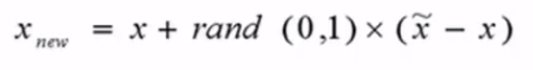
• （1）对于少数类中每一个样本x，找出离它最近的N个样本，再随机生成0~1的数 * 欧式距离+x原本的距离，得到新的样本点
• （2）根据样本不平衡比例设置一个采样比例以确定采样倍率N
  
• 删除class列，对特征求欧式距离从而生成数据
• 切分数据
• 对SMOTE实例化，然后fit特征和标签

import pandas as pd
from imblearn.over_sampling import SMOTE
from sklearn.ensemble import RandomForestClassifier
from sklearn.metrics import confusion_matrix
from sklearn.model_selection import train_test_split


credit_cards=pd.read_csv('creditcard.csv')

columns=credit_cards.columns
# The labels are in the last column ('Class'). Simply remove it to obtain features columns

features_columns=columns.delete(len(columns)-1)

features=credit_cards[features_columns]
labels=credit_cards['Class']

features_train, features_test, labels_train, labels_test = train_test_split(features, 
                                                                            labels, 
                                                                            test_size=0.2, 
                                                                            random_state=0)
                                                                           
oversampler=SMOTE(random_state=0)
os_features,os_labels=oversampler.fit_sample(features_train,labels_train)

len(os_labels[os_labels==1])

已经构建了二十多万的数据量：

227454

从SMOTE数据集训练的模型，recall相差不大，但精度有很大的提高，相比于之前的误判数量大幅减小

lr = LogisticRegression(C = best_c, penalty = 'l1')
lr.fit(os_features,os_labels.values.ravel())
y_pred = lr.predict(features_test.values)

# Compute confusion matrix
cnf_matrix = confusion_matrix(labels_test,y_pred)
np.set_printoptions(precision=2)

print("Recall metric in the testing dataset: ", cnf_matrix[1,1]/(cnf_matrix[1,0]+cnf_matrix[1,1]))

# Plot non-normalized confusion matrix
class_names = [0,1]
plt.figure()
plot_confusion_matrix(cnf_matrix
                      , classes=class_names
                      , title='Confusion matrix')
plt.show()