多元线性回归示例（原生实现、sklearn实现）

版权声明：本文为博主原创文章，未经博主允许不得转载。 https://blog.csdn.net/alionsss/article/details/86820485

0. 原始数据准备

0.1 数据

# 房屋面积、房间数
x_data = np.array(
    [[100, 4],
     [ 50, 1],
     [100, 4],
     [100, 3],
     [ 50, 2],
     [ 80, 2],
     [ 75, 3],
     [ 65, 4],
     [ 90, 3],
     [ 90, 2]])
# 房屋价格（单位是百万）
y_data = np.array([9.3, 4.8, 8.9, 6.5, 4.2, 6.2, 7.4, 6.0,  7.6, 6.1])
print(x_data)
print(y_data)

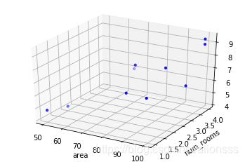
0.2 作图展示

ax = plt.figure().add_subplot(111, projection = "3d")
ax.scatter(x_data[:, 0], x_data[:, 1], y_data, c = "b", marker = 'o', s = 10)
ax.set_xlabel("area")
ax.set_ylabel("num_rooms")
plt.show()

1. Python原生实现

1.1 导包

import numpy as np
import matplotlib.pyplot as plt
from mpl_toolkits.mplot3d import Axes3D

1.2 计算均方差

def compute_mse(b, w, x_data, y_data):
    """
    求均方差
    :param b: 截距
    :param w1: 斜率1
    :param w2: 斜率2
    :param x_data: 特征数据
    :param y_data: 标签数据
    """
    
    total_error = 0.0
    for i in range(0, len(x_data)):
        total_error += (y_data[i] - (b + w1 * x_data[i, 0] + w2 * x_data[i, 1])) ** 2
    return total_error / len(x_data)

1.3 梯度下降

def run_gradient_descent(x_data, y_data, b, w, learn_rate, epochs):
    """
    运行梯度下降
    :param x_data: 待训练的特征数据
    :param y_data: 标签数据
    :param b: 截距
    :param w1: 斜率1
    :param w2: 斜率2
    :param learn_rate: 学习曲率
    :param epochs: 训练次数
    """
    
    m = float(len(x_data))
    for i in range(epochs):
        b_grad = 0 # 损失（代价）函数对b的梯度
        w1_grad = 0 # 损失（代价）函数对w1的梯度
        w2_grad = 0 # 损失（代价）函数对w2的梯度
        for j in range(0, len(x_data)):
            b_grad += (1/m) * ((b + w1 * x_data[j, 0] + w2 * x_data[j, 1]) - y_data[j])
            w1_grad += (1/m) * ((b + w1 * x_data[j, 0] + w2 * x_data[j, 1]) - y_data[j]) * x_data[j, 0]
            w2_grad += (1/m) * ((b + w1 * x_data[j, 0] + w2 * x_data[j, 1]) - y_data[j]) * x_data[j, 1]
        # 根据梯度和学习曲率修正截距b和斜率w1、w2
        b -= learn_rate * b_grad
        w1 -= learn_rate * w1_grad
        w2 -= learn_rate * w2_grad
        if i % 100 == 0:
        	# 每100次作图一次
            print("epochs:", i)
            ax = plt.figure().add_subplot(111, projection = "3d")
            ax.scatter(x_data[:, 0], x_data[:, 1], y_data, c = "b", marker = 'o', s = 10)
            x0 = x_data[:, 0]
            x1 = x_data[:, 1]
            x0, x1 = np.meshgrid(x0, x1)
            z = b + w1 * x0 + w2 * x1
            ax.plot_surface(x0, x1, z, color = "r")
            ax.set_xlabel("area")
            ax.set_ylabel("num_rooms")
            ax.set_zlabel("price")
            plt.show()
            print("mse: ", compute_mse(b, w1, w2, x_data, y_data))
            print("------------------------------------------------------------------------------------------------------------")
    return b, w1, w2

1.4 开始运行

learn_rate = 0.0001
b = 0
w1 = 0
w2 = 0
epochs = 1000

print("Start args: b = {0}, w1 = {1}, w2 = {2}, mse = {3}".format(b, w1, w2, compute_mse(b, w1, w2, x_data, y_data)))
print("Running...")
b, w1, w2 = run_gradient_descent(x_data, y_data, b, w1, w2, learn_rate, epochs)
print("Finish args: iterations = {0}  b = {1}, w1 = {2}, w2 = {3}, mse = {4}".format(epochs, b, w1, w2, compute_mse(b, w1, w2, x_data, y_data)))

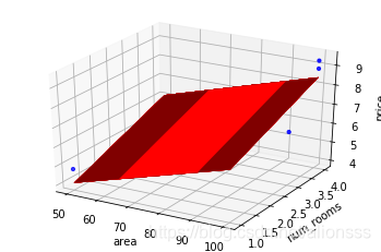
1.5 回归最终结果作图

ax = plt.figure().add_subplot(111, projection = "3d")
ax.scatter(x_data[:, 0], x_data[:, 1], y_data, c = "b", marker = 'o', s = 10)
x0 = x_data[:, 0]
x1 = x_data[:, 1]
x0, x1 = np.meshgrid(x0, x1)
z = b + w1 * x0 + w2 * x1
ax.plot_surface(x0, x1, z, color = "r")
ax.set_xlabel("area")
ax.set_ylabel("num_rooms")
ax.set_zlabel("price")
plt.show()

2. sklearn实现

2.1 导包

import numpy as np
from sklearn.linear_model import LinearRegression
from mpl_toolkits.mplot3d import Axes3D
import matplotlib.pyplot as plt

2.2 建模与训练

# 建立模型
model = LinearRegression()
# 开始训练
model.fit(x_data, y_data)

2.3 结果展示

# 斜率
print("coefficients: ", model.coef_)
w1 = model.coef_[0]
w2 = model.coef_[1]

# 截距
print("intercept: ", model.intercept_)
b = model.intercept_

# 测试
x_test = [[90, 3]]
predict = model.predict(x_test)
print("predict: ", predict)

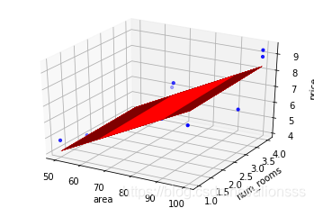
2.4 回归最终结果作图

ax = plt.figure().add_subplot(111, projection = "3d")
ax.scatter(x_data[:, 0], x_data[:, 1], y_data, c = "b", marker = 'o', s = 10)
x0 = x_data[:, 0]
x1 = x_data[:, 1]
x0, x1 = np.meshgrid(x0, x1)
z = b + w1 * x0 + w2 * x1
ax.plot_surface(x0, x1, z, color = "r")
ax.set_xlabel("area")
ax.set_ylabel("num_rooms")
ax.set_zlabel("price")
plt.show()