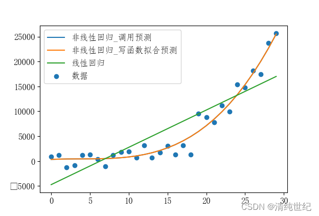
代码:
import pandas as pd
import numpy as np
import matplotlib
import random
from matplotlib import pyplot as plt
from sklearn.preprocessing import PolynomialFeatures
from sklearn.linear_model import LinearRegression
# 创建虚拟数据
x = np.array(range(30))
temp_y = 10 + 2 * x + x ** 2 + x ** 3
y = temp_y + 1500 * np.random.normal(size=30) # 添加噪声
x = x.reshape(30, 1)
y = y.reshape(30, 1)
# 线性回归
clf1 = LinearRegression()
clf1.fit(x, y)
y_l = clf1.predict(x) # 线性回归预测值
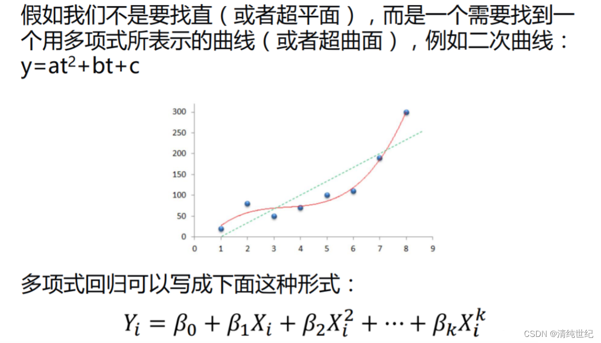
# 非线性回归
ployfeat = PolynomialFeatures(degree=3) # 根据degree的值转换为相应的多项式(非线性回归)
x_p = ployfeat.fit_transform(x)
clf2 = LinearRegression()
clf2.fit(x_p, y)
print("线性回归方程为: y = {} + {}x".format(clf1.intercept_[0],clf1.coef_[0,0]))
print("非线性回归曲线方程为 y = {}+{}x+{}x^2+{}x^3".format(clf2.intercept_[0],clf2.coef_[0,1],clf2.coef_[0,2],clf2.coef_[0,3]))
def f(x):
return clf2.intercept_[0]+clf2.coef_[0,1]*(x**1)+clf2.coef_[0,2]*(x**2)+clf2.coef_[0,3]*(x**3)
font={"family":"FangSong",'size':12}
matplotlib.rc("font",**font)
plt.plot(x, clf2.predict(x_p),label="非线性回归_调用预测")
plt.plot(x, f(x),label="非线性回归_写函数拟合预测")
plt.plot(x, y_l,label="线性回归")
plt.scatter(x, y,label="数据")
plt.legend()
plt.show()