sklearn实现非线性逻辑回归
前言: 上一篇博文,我使用python实现了非线性逻辑回归的梯度下降算法进行分类,看上去比较复杂,这篇博文将利用sklearn包进行非线性逻辑回归的实现,非线性实现的思想也是通处理样本数据将非线性转为线性,具体思路看我的这篇博文
一、sklearn实现非线性逻辑回归Demo
import matplotlib.pyplot as plt
import numpy as np
from sklearn import linear_model
from sklearn.metrics import classification_report
from sklearn.datasets import make_gaussian_quantiles
from sklearn.preprocessing import PolynomialFeatures

# 生成2维正态分布,生成的数据按分位数分为两类,500个样本,2个样本特征
# 可以生成两类或者多类数据
x_data, y_data = make_gaussian_quantiles(n_samples=500, n_features=2, n_classes=2)

# 定义多项式回归,degree的值可以调节多项式的特征
poly_reg = PolynomialFeatures(degree=3)  # 得到非线性方程y = theta0+theta1*x1+theta2*x1^2+theta3*x1*x2+theta4*x^2所需的样本数据
# 特征处理(获取多项式相应特征所对应的样本数据)
x_poly = poly_reg.fit_transform(x_data)

# 训练模型
model = linear_model.LogisticRegression()
model.fit(x_poly, y_data)

# 获取数据值所在的范围
x_min, x_max = x_data[:, 0].min() - 1, x_data[:, 0].max() + 1
y_min, y_max = x_data[:, 1].min() - 1, x_data[:, 1].max() + 1

# 生成网格矩阵
xx, yy = np.meshgrid(np.arange(x_min, x_max, 0.02), np.arange(y_min, y_max, 0.02))
# 测试点的预测值
z = model.predict(poly_reg.fit_transform(np.c_[xx.ravel(), yy.ravel()]))
for i in range(len(z)):
    if z[i] > 0.5:
        z[i] = 1
    else:
        z[i] = 0

z = z.reshape(xx.shape)
# 绘制等高线图
cs = plt.contourf(xx, yy, z)
plt.scatter(x_data[:, 0], x_data[:, 1], c=y_data)

# 计算准确率,召回率,F1值
print(classification_report(y_data, model.predict(x_poly)))
print('score:', model.score(x_poly, y_data))
plt.show()
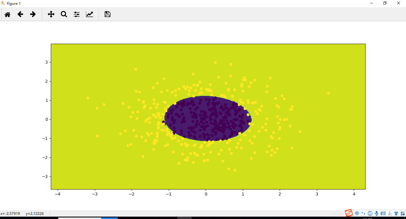
二、执行结果
                  precision    recall  f1-score   support

	           		0       0.97      0.99      0.98       250
           			1       0.99      0.97      0.98       250

   micro avg       0.98      0.98      0.98       500
   macro avg       0.98      0.98      0.98       500
weighted avg       0.98      0.98      0.98       500