深度学习（6）——循环神经网络RNN+LSTM

目录

一、概念

1.1 RNN

1.2 LSTM（long short-term memory）

二、RNN变种

三、自然语言建模

四、时间序列预测

---

一、概念

1.1 RNN

主要用来处理和预测序列数据。特点：隐藏层的输入不仅包括输入层的输出，还包括上一时刻隐藏层的输出，即当前时刻的状态是根据上一时刻的状态和当前的输入共同决定的。

前向传播计算过程

实现过程

# -*- coding: utf-8 -*-
import tensorflow as tf
import numpy as np
#初始状态
X=[1,2]
state=[0.0,0.0]
#定义不同部分的权重
w_state=np.asarray([[0.1,0.2],[0.3,0.4]])
w_input=np.asarray([0.5,0.6])
b=np.asarray([0.1,-0.1])
#定义用于输出的全连接层参数
w_output=np.asarray([[1.0],[2.0]])
b_output=0.1

for i in range(len(X)):
    before_activation=np.dot(state,w_state)+X[i]*w_input+b
    state=np.tanh(before_activation)
    #输出每一时刻的信息
    final_output=np.dot(state,w_output)+b_output
    print("before activation:",before_activation)
    print("state:",state)
    print("output:",final_output)

1.2 LSTM（long short-term memory）

解决长期依赖，例如当前预测位置和相关信息之间的文本间隔有可能很长，也有可能很短。

 特点：依靠门结构让信息有选择性的影响RNN中每个时刻的状态。

遗忘门：根据当前的输入、上一时刻 的状态和上一时刻的输出共同决定需要被遗忘的部分

输入门：在循环神经网络忘记了部分之前的状态后，从当前的输入中补充最新的记忆，还是根据当前的输入，上一时刻的状态和输出共同决定哪些部分进入当前时刻

输出门：根据当前的输入、当前的状态和上一时刻的输出决定此刻的输出。

具体实现：使用sigmoid神经网络和按位做乘法。具体门的公式可以参考论文：long short-term memory

# 伪代码
#tensorflow中有简单的实现命令
lstm=rnn_cell.BasicLSTMCell(lstm_hidden_size)

#初始状态为全0数组
state=lstm.zero_state(batch_size,tf.float32)

loss=0.0
for i in range(num_steps):
	if i>0:
		#获取需要使用的变量
		tf.get_variabel_scope().reuse_variables()
		#将当前输入和前一时刻状态传入定义的LSTM结构获取当前输出和更新后的状态
		lstm_output, state=lstm(current_input, state)
		#计算当前时刻的lstm结构的输出经过一个全连接神经网络后的最后的输出
		final_output=fully_connected(lstm_output)
		#计算当前的损失
		loss+=calc_loss(final_output,expected_output)

二、RNN变种

双向循环神经网络（bidirectional RNN）：由两个RNN上下叠加在一起组成，输出由这两个RNN共同决定

双层循环神经网络（deepRNN）：将每个时刻上的循环体重复多次，和CNN类似，每一层循环体的参数一致，不同层中的参数可以不同

RNN中的dropout

CNN只在最后的全连接层中使用dropout

RNN一般只在不同层循环体结构之间使用，而不在同一层的循环体结构之间使用

三、自然语言建模

使用PTB文本数据集（Penn Treebank Dataset）

tensorflow提供了两个很方便的函数对ptb数据进行预处理

ptb_raw_data()读取数据

ptb_producer()进行数据截断

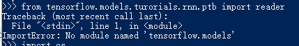
from tensorflow.models.rnn.ptb import reader
data_path="D:\MyData\MyProgram\simple-examples\data"
train_data,valid_data,test_data,_=reader.ptb_raw_data(data_path)
print(len(train_data))
print(train_data[:100])

#将训练数据组织成batch大小为4，截断长度为5的数据组
result=reader.ptb_producer(train_data,4,5)
with tf.Session() as sess:
    coord = tf.train.Coordinator()
    threads = tf.train.start_queue_runners(sess=sess, coord=coord)
    for i in range(3):
        x, y = sess.run(result)
        print ("X%d: "%i, x)
        print ("Y%d: "%i, y)
    coord.request_stop()
    coord.join(threads)

 读取数据集的时候碰到了一个问题，提示我的tensorflow下面没有models。

于是我就去下载了models文件，解压到tensorflow文件夹下，https://github.com/tensorflow/models。

接着提示我没有reader

把指定路径下的文件中的路径修改一下就可以了

也就是把reader和util的路径修改一下 

下面是一个完整的自然语言处理的例子

# -*- coding: utf-8 -*-
import numpy as np
import tensorflow as tf
from tensorflow.models.rnn.ptb import reader

#定义参数
DATA_PATH="D:\MyData\MyProgram\simple-examples\data"
HIDDEN_SIZE = 200
NUM_LAYERS = 2
VOCAB_SIZE = 10000

LEARNING_RATE = 1.0
TRAIN_BATCH_SIZE = 20
TRAIN_NUM_STEP = 35

EVAL_BATCH_SIZE = 1
EVAL_NUM_STEP = 1
NUM_EPOCH = 2
KEEP_PROB = 0.5
MAX_GRAD_NORM = 5

#定义一个类来描述模型结构
class PTBModel(object):
    def __init__(self, is_training, batch_size, num_steps):
        
        self.batch_size = batch_size
        self.num_steps = num_steps
        
        # 定义输入层。
        self.input_data = tf.placeholder(tf.int32, [batch_size, num_steps])
        self.targets = tf.placeholder(tf.int32, [batch_size, num_steps])
        
        # 定义使用LSTM结构及训练时使用dropout。
        lstm_cell = tf.contrib.rnn.BasicLSTMCell(HIDDEN_SIZE)
        if is_training:
            lstm_cell = tf.contrib.rnn.DropoutWrapper(lstm_cell, output_keep_prob=KEEP_PROB)
        cell = tf.contrib.rnn.MultiRNNCell([lstm_cell]*NUM_LAYERS)
        
        # 初始化最初的状态。
        self.initial_state = cell.zero_state(batch_size, tf.float32)
        embedding = tf.get_variable("embedding", [VOCAB_SIZE, HIDDEN_SIZE])
        
        # 将原本单词ID转为单词向量。
        inputs = tf.nn.embedding_lookup(embedding, self.input_data)
        
        if is_training:
            inputs = tf.nn.dropout(inputs, KEEP_PROB)

        # 定义输出列表。
        outputs = []
        state = self.initial_state
        with tf.variable_scope("RNN"):
            for time_step in range(num_steps):
                if time_step > 0: tf.get_variable_scope().reuse_variables()
                cell_output, state = cell(inputs[:, time_step, :], state)
                outputs.append(cell_output) 
        output = tf.reshape(tf.concat(outputs, 1), [-1, HIDDEN_SIZE])
        weight = tf.get_variable("weight", [HIDDEN_SIZE, VOCAB_SIZE])
        bias = tf.get_variable("bias", [VOCAB_SIZE])
        logits = tf.matmul(output, weight) + bias
        
        # 定义交叉熵损失函数和平均损失。
        loss = tf.contrib.legacy_seq2seq.sequence_loss_by_example(
            [logits],
            [tf.reshape(self.targets, [-1])],
            [tf.ones([batch_size * num_steps], dtype=tf.float32)])
        self.cost = tf.reduce_sum(loss) / batch_size
        self.final_state = state
        
        # 只在训练模型时定义反向传播操作。
        if not is_training: return
        trainable_variables = tf.trainable_variables()

        # 控制梯度大小，定义优化方法和训练步骤。
        grads, _ = tf.clip_by_global_norm(tf.gradients(self.cost, trainable_variables), MAX_GRAD_NORM)
        optimizer = tf.train.GradientDescentOptimizer(LEARNING_RATE)
        self.train_op = optimizer.apply_gradients(zip(grads, trainable_variables))
		
#使用给定的模型model在数据data上运行train_op并返回在全部数据上的perplexity值
def run_epoch(session, model, data, train_op, output_log, epoch_size):
    total_costs = 0.0
    iters = 0
    state = session.run(model.initial_state)

    # 训练一个epoch。
    for step in range(epoch_size):
        x, y = session.run(data)
        cost, state, _ = session.run([model.cost, model.final_state, train_op],
                                        {model.input_data: x, model.targets: y, model.initial_state: state})
        total_costs += cost
        iters += model.num_steps

        if output_log and step % 100 == 0:
            print("After %d steps, perplexity is %.3f" % (step, np.exp(total_costs / iters)))
    return np.exp(total_costs / iters)
	
def main():
    train_data, valid_data, test_data, _ = reader.ptb_raw_data(DATA_PATH)

    # 计算一个epoch需要训练的次数
    train_data_len = len(train_data)
    train_batch_len = train_data_len // TRAIN_BATCH_SIZE
    train_epoch_size = (train_batch_len - 1) // TRAIN_NUM_STEP

    valid_data_len = len(valid_data)
    valid_batch_len = valid_data_len // EVAL_BATCH_SIZE
    valid_epoch_size = (valid_batch_len - 1) // EVAL_NUM_STEP

    test_data_len = len(test_data)
    test_batch_len = test_data_len // EVAL_BATCH_SIZE
    test_epoch_size = (test_batch_len - 1) // EVAL_NUM_STEP

    initializer = tf.random_uniform_initializer(-0.05, 0.05)
    with tf.variable_scope("language_model", reuse=None, initializer=initializer):
        train_model = PTBModel(True, TRAIN_BATCH_SIZE, TRAIN_NUM_STEP)

    with tf.variable_scope("language_model", reuse=True, initializer=initializer):
        eval_model = PTBModel(False, EVAL_BATCH_SIZE, EVAL_NUM_STEP)

    # 训练模型。
    with tf.Session() as session:
        tf.global_variables_initializer().run()

        train_queue = reader.ptb_producer(train_data, train_model.batch_size, train_model.num_steps)
        eval_queue = reader.ptb_producer(valid_data, eval_model.batch_size, eval_model.num_steps)
        test_queue = reader.ptb_producer(test_data, eval_model.batch_size, eval_model.num_steps)

        coord = tf.train.Coordinator()
        threads = tf.train.start_queue_runners(sess=session, coord=coord)

        for i in range(NUM_EPOCH):
            print("In iteration: %d" % (i + 1))
            run_epoch(session, train_model, train_queue, train_model.train_op, True, train_epoch_size)

            valid_perplexity = run_epoch(session, eval_model, eval_queue, tf.no_op(), False, valid_epoch_size)
            print("Epoch: %d Validation Perplexity: %.3f" % (i + 1, valid_perplexity))

        test_perplexity = run_epoch(session, eval_model, test_queue, tf.no_op(), False, test_epoch_size)
        print("Test Perplexity: %.3f" % test_perplexity)

        coord.request_stop()
        coord.join(threads)

if __name__ == "__main__":
    main()

四、时间序列预测

使用RNN来预测正弦函数

# -*- coding: utf-8 -*-

import numpy as np
import tensorflow as tf
import matplotlib.pyplot as plt

#定义网络参数
HIDDEN_SIZE = 30                            # LSTM中隐藏节点的个数。
NUM_LAYERS = 2                              # LSTM的层数。
TIMESTEPS = 10                              # 循环神经网络的训练序列长度。
TRAINING_STEPS = 10000                      # 训练轮数。
BATCH_SIZE = 32                             # batch大小。
TRAINING_EXAMPLES = 10000                   # 训练数据个数。
TESTING_EXAMPLES = 1000                     # 测试数据个数。
SAMPLE_GAP = 0.01                           # 采样间隔。

#产生正弦数据
def generate_data(seq):
    X = []
    y = []
    # 序列的第i项和后面的TIMESTEPS-1项合在一起作为输入；第i + TIMESTEPS项作为输
    # 出。即用sin函数前面的TIMESTEPS个点的信息，预测第i + TIMESTEPS个点的函数值。
    for i in range(len(seq) - TIMESTEPS):
        X.append([seq[i: i + TIMESTEPS]])
        y.append([seq[i + TIMESTEPS]])
    return np.array(X, dtype=np.float32), np.array(y, dtype=np.float32)  

# 用正弦函数生成训练和测试数据集合。
test_start = (TRAINING_EXAMPLES + TIMESTEPS) * SAMPLE_GAP
test_end = test_start + (TESTING_EXAMPLES + TIMESTEPS) * SAMPLE_GAP
train_X, train_y = generate_data(np.sin(np.linspace(
    0, test_start, TRAINING_EXAMPLES + TIMESTEPS, dtype=np.float32)))
test_X, test_y = generate_data(np.sin(np.linspace(
    test_start, test_end, TESTING_EXAMPLES + TIMESTEPS, dtype=np.float32)))
	
	
#定义网络结构和优化步骤
def lstm_model(X, y, is_training):
    # 使用多层的LSTM结构。
    cell = tf.nn.rnn_cell.MultiRNNCell([
        tf.nn.rnn_cell.BasicLSTMCell(HIDDEN_SIZE) 
        for _ in range(NUM_LAYERS)])    

    # 使用TensorFlow接口将多层的LSTM结构连接成RNN网络并计算其前向传播结果。
    outputs, _ = tf.nn.dynamic_rnn(cell, X, dtype=tf.float32)
    output = outputs[:, -1, :]

    # 对LSTM网络的输出再做加一层全链接层并计算损失。注意这里默认的损失为平均
    # 平方差损失函数。
    predictions = tf.contrib.layers.fully_connected(
        output, 1, activation_fn=None)
    
    # 只在训练时计算损失函数和优化步骤。测试时直接返回预测结果。
    if not is_training:
        return predictions, None, None
        
    # 计算损失函数。
    loss = tf.losses.mean_squared_error(labels=y, predictions=predictions)

    # 创建模型优化器并得到优化步骤。
    train_op = tf.contrib.layers.optimize_loss(
        loss, tf.train.get_global_step(),
        optimizer="Adagrad", learning_rate=0.1)
    return predictions, loss, train_op
	
#定义测试方法
def run_eval(sess, test_X, test_y):
    # 将测试数据以数据集的方式提供给计算图。
    ds = tf.data.Dataset.from_tensor_slices((test_X, test_y))
    ds = ds.batch(1)
    X, y = ds.make_one_shot_iterator().get_next()
    
    # 调用模型得到计算结果。这里不需要输入真实的y值。
    with tf.variable_scope("model", reuse=True):
        prediction, _, _ = lstm_model(X, [0.0], False)
    
    # 将预测结果存入一个数组。
    predictions = []
    labels = []
    for i in range(TESTING_EXAMPLES):
        p, l = sess.run([prediction, y])
        predictions.append(p)
        labels.append(l)

    # 计算rmse作为评价指标。
    predictions = np.array(predictions).squeeze()
    labels = np.array(labels).squeeze()
    rmse = np.sqrt(((predictions - labels) ** 2).mean(axis=0))
    print("Root Mean Square Error is: %f" % rmse)
    
    #对预测的sin函数曲线进行绘图。
    plt.figure()
    plt.plot(predictions, label='predictions')
    plt.plot(labels, label='real_sin')
    plt.legend()
    plt.show()
	
#执行训练和测试
# 将训练数据以数据集的方式提供给计算图。
ds = tf.data.Dataset.from_tensor_slices((train_X, train_y))
ds = ds.repeat().shuffle(1000).batch(BATCH_SIZE)
X, y = ds.make_one_shot_iterator().get_next()

# 定义模型，得到预测结果、损失函数，和训练操作。
with tf.variable_scope("model"):
    _, loss, train_op = lstm_model(X, y, True)
    
with tf.Session() as sess:
    sess.run(tf.global_variables_initializer())
    
    # 测试在训练之前的模型效果。
    print ("Evaluate model before training.")
    run_eval(sess, test_X, test_y)
    
    # 训练模型。
    for i in range(TRAINING_STEPS):
        _, l = sess.run([train_op, loss])
        if i % 1000 == 0:
            print("train step: " + str(i) + ", loss: " + str(l))
    
    # 使用训练好的模型对测试数据进行预测。
    print ("Evaluate model after training.")
    run_eval(sess, test_X, test_y)