文章目录
写在前面
因为近期要做一些金融股票预测相关的项目课题,最近两天着手看了一下 R N N \rm RNN RNN和 L S T M \rm LSTM LSTM,以前也零零碎碎的看过几次,但都被它庞杂的网络结构和公式吓退了,这次终于静下心来研究了一下这两个网络,并且也亲自用手推导了一下它们的反向传播过程,也辛辛苦苦亲手打了很多公式、画了很多图,花了很长时间,绝对超级详细,只要静下心来,我相信谁都能看懂它们的工作机制尤其是是 L S T M \rm LSTM LSTM,最终写下这片文章,一是为更多的人透析其原理提供便利,二是方便自己回过头来复习。里面的内容是自己的理解并结合相关参考资料做的一些笔记,走过路过的朋友们一键三连互关走起来,互相学习,共同促进!再次感谢大佬们的文章和视频!
循环神经网络RNN
引言
循环神经网络 ( R e c u r r e n t N e u r a l N e t w o r k ) (\rm Recurrent \ Neural \ Network) (Recurrent Neural Network)是指随着时间推移,重复发生的结构。在自然语言处理、语音图像处理等多个领域都有着广泛的应用,它是一种处理序列数据的神经网络模型。传统的神经网络包含输入层、隐含层、输出层,通过激活函数来控制输出,层层之间通过权值进行连接,神经网络训练的终极目的就是学习到一组权值,用来处理新数据,从而达到我们要求。比如卷积神经网络 ( C N N ) (\rm CNN) (CNN),它通过前向传播计算出的输出只考虑前一个输入的影响而不考虑其他时刻输入的影响。
循环神经网络与传统神经网络最大的不同就是,拥有"记忆功能"——可以用来处理基于序列的数据。例如,你要预测一个句子的下一个单词是什么,一般需要用到前面的单词,因为句子中的单词是并不是脱离上下文环境而存在的,我们必须要考虑其所在的上下文环境。也就是说, R N N \rm RNN RNN处理的数据当前时刻的输出与前面时刻的输出也有关系。
网络结构
R N N \rm RNN RNN的记忆功能具体表现为网络会对前面的信息进行记忆并应用于当前输出的计算中。因此隐藏层之间产生了连接,并且隐藏层的输入不仅包括输入层的输入值,还包括上一时刻隐藏层的输出值。
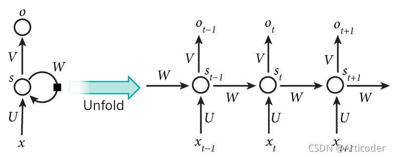
从上述图中可以看出权重矩阵 W W W作用于每一个隐藏层的神经元。其中 x t x_t xt表示当前 t t t的输入层输入值, s t s_t st表示时刻 t t t的隐藏层输出值(下文中用 h t h_t ht表示隐藏层的输出值), o t o_t ot则表示时刻 t t t的输出值, U U U表示输入层的权值, V V V表示输出层的权值。
权值共享:通过网络结构可以看出, U , V , W U,V,W U,V,W是所有特征共享的一组参数,其优点就是面对不同的输入,能学到不同的相应的结果;减少了训练参数的数量;输入和输出数据在不同的例子中长度可以不同。
前向传播
从网络结构中我们可以看出, R N N \rm RNN RNN的主要计算的参数就是隐藏层的输出值和输出层的值。
h t = f ( U x t + W h t − 1 ) o t = g ( V h t ) \begin{aligned} h_t &= f(Ux_t + Wh_{t - 1}) \\ o_t &= g(Vh_t) \end{aligned} htot=f(Uxt+Wht−1)=g(Vht)
在上述计算过程中,函数 f , g f, g f,g为激活函数, f f f一般取 tanh \tanh tanh函数, g g g一般取 s o f t m a x \rm softmax softmax函数。
通过反复代入
o t = g ( V h t ) = g V ( f ( U x t + W h t − 1 ) ) = g V ( f ( U x t + W f ( U x t − 1 + W h t − 2 ) ) ) = g V ( f ( U x t + W f ( U x t − 1 + W f ( U x t − 2 + W h t − 3 ) ) ) ) = ⋯ \begin{aligned} o_t &= g(V h_t) \\ &= gV(f(Ux_t + Wh_{t - 1})) \\ &= gV(f(Ux_t + Wf(Ux_{t -1} + Wh_{t - 2}))) \\ &= gV(f(Ux_t + Wf(Ux_{t -1} + Wf(Ux_{t - 2} + Wh_{t-3})))) \\ &= \cdots \end{aligned} ot=g(Vht)=gV(f(Uxt+Wht−1))=gV(f(Uxt+Wf(Uxt−1+Wht−2)))=gV(f(Uxt+Wf(Uxt−1+Wf(Uxt−2+Wht−3))))=⋯
由此可见, t t t时刻的输出与 x t , x t − 1 , x t − 2 , x t − 3 , ⋯ x_t, x_{t-1}, x_{t-2},x_{t-3}, \cdots xt,xt−1,xt−2,xt−3,⋯都相关。
此处省去偏置值 b b b,一般是需要加该值的。
损失函数
单个时间步损失可以根据任务类型定义,使用较为广泛的是交叉熵损失 ( C E ) (\rm CE) (CE),即
L C E = − ( y t ln o t + ( 1 − y t ) ln ( 1 − o t ) ) L_{\rm CE} = - (y_t \ln o_t + (1 - y_t) \ln (1 - o_t)) LCE=−(ytlnot+(1−yt)ln(1−ot))
整个时间序列的损失就是单个时间步的损失之和,即
L = ∑ t L C E L = \sum_t L_{\rm CE} L=t∑LCE
其中, y t y_t yt表示时刻 t t t的真实标签值, o t o_t ot表示时刻 t t t模型预测输出值。
反向传播
从前向传播的过程中,可以看出只需要对三个权值 U , V , W U,V,W U,V,W进行优化即可,因此分别对其求梯度。
参数优化
-
对参数 V V V求偏导
∂ L ∂ V = ∑ t ∂ L t ∂ o t ∂ o t ∂ V \frac{\partial{L}}{\partial{V}} = \sum_{t} \frac{\partial{L_t}}{\partial{o_t}} \frac{\partial{o_t}} {\partial{V}} ∂V∂L=t∑∂ot∂Lt∂V∂ot
其中还要对复合函数(激活函数)求导。 -
对参数 W W W求偏导
对该参数涉及到之前时刻的信息,求导相对比较复杂,因此假设在 t = 3 t= 3 t=3时刻,利用前面时刻的数据对 W W W求导,即
∂ L 3 ∂ W = ∂ L 3 ∂ o 3 ∂ o 3 ∂ h 3 ( ∂ h 3 ∂ W + ∂ h 3 ∂ h 2 ∂ h 2 ∂ W + ∂ h 3 ∂ h 2 ∂ h 2 ∂ h 1 ∂ h 1 ∂ W ) = ∂ L t ∂ o t ∂ o t ∂ h t ∑ j = 1 t [ ( ∏ i = j + 1 t ∂ h i ∂ h i − 1 ) ∂ h j ∂ W ] \begin{aligned} \frac{\partial{L_3}}{\partial{W}} &= \frac{\partial{L_3}}{\partial{o_3}} \frac{\partial{o_3}}{\partial{h_3}} (\frac{\partial{h_3}}{\partial{W}} + \frac{\partial{h_3}}{\partial{h_2}} \frac{\partial{h_2}}{\partial{W}} + \frac{\partial{h_3}}{\partial{h_2}} \frac{\partial{h_2}}{\partial{h_1}} \frac{\partial{h_1}}{\partial{W}}) \\ &= \frac{\partial{L_t}}{\partial{o_t}} \frac{\partial{o_t}}{\partial{h_t}} \sum_{j=1}^t \left[ \left(\prod_{i = j+1}^t \frac{\partial{h_{i}}}{\partial{h_{i - 1}}}\right) \frac{\partial{h_j}}{\partial{W}}\right] \end{aligned} ∂W∂L3=∂o3∂L3∂h3∂o3(∂W∂h3+∂h2∂h3∂W∂h2+∂h2∂h3∂h1∂h2∂W∂h1)=∂ot∂Lt∂ht∂otj=1∑t[(i=j+1∏t∂hi−1∂hi)∂W∂hj]
-
对参数 U U U求偏导
假设同上。故有
∂ L 3 ∂ W = ∂ L 3 ∂ o 3 ∂ o 3 ∂ h 3 ( ∂ h 3 ∂ U + ∂ h 3 ∂ h 2 ∂ h 2 ∂ U + ∂ h 3 ∂ h 2 ∂ h 2 ∂ h 1 ∂ h 1 ∂ U ) = ∂ L t ∂ o t ∂ o t ∂ h t ∑ j = 1 t [ ( ∏ i = j + 1 t ∂ h i ∂ h i − 1 ) ∂ h j ∂ U ] \begin{aligned} \frac{\partial{L_3}}{\partial{W}} &= \frac{\partial{L_3}}{\partial{o_3}} \frac{\partial{o_3}}{\partial{h_3}} (\frac{\partial{h_3}}{\partial{U}} + \frac{\partial{h_3}}{\partial{h_2}} \frac{\partial{h_2}}{\partial{U}} + \frac{\partial{h_3}}{\partial{h_2}} \frac{\partial{h_2}}{\partial{h_1}} \frac{\partial{h_1}}{\partial{U}}) \\ &= \frac{\partial{L_t}}{\partial{o_t}} \frac{\partial{o_t}}{\partial{h_t}} \sum_{j=1}^t \left[ \left(\prod_{i = j+1}^t \frac{\partial{h_{i}}}{\partial{h_{i - 1}}}\right) \frac{\partial{h_j}}{\partial{U}}\right] \end{aligned} ∂W∂L3=∂o3∂L3∂h3∂o3(∂U∂h3+∂h2∂h3∂U∂h2+∂h2∂h3∂h1∂h2∂U∂h1)=∂ot∂Lt∂ht∂otj=1∑t[(i=j+1∏t∂hi−1∂hi)∂U∂hj]
梯度消失或爆炸
在参数优化过程中,随着时间的不断累积,对参数 U , W U,W U,W的优化过程就会出现梯度累乘,此间要对函数 f f f求导,因此有
∏ i = j + 1 t ∂ h i ∂ h i − 1 = ∏ i = j + 1 t f ′ ⋅ W \prod_{i = j+1}^t \frac{\partial{h_{i}}}{\partial{h_{i - 1}}} = \prod_{i = j+1}^t f' \cdot W i=j+1∏t∂hi−1∂hi=i=j+1∏tf′⋅W
就会导致激活函数的累乘,由于激活函数通常为 tanh \tanh tanh或者 s i g m o i d \rm sigmoid sigmoid,其函数和导数图像为
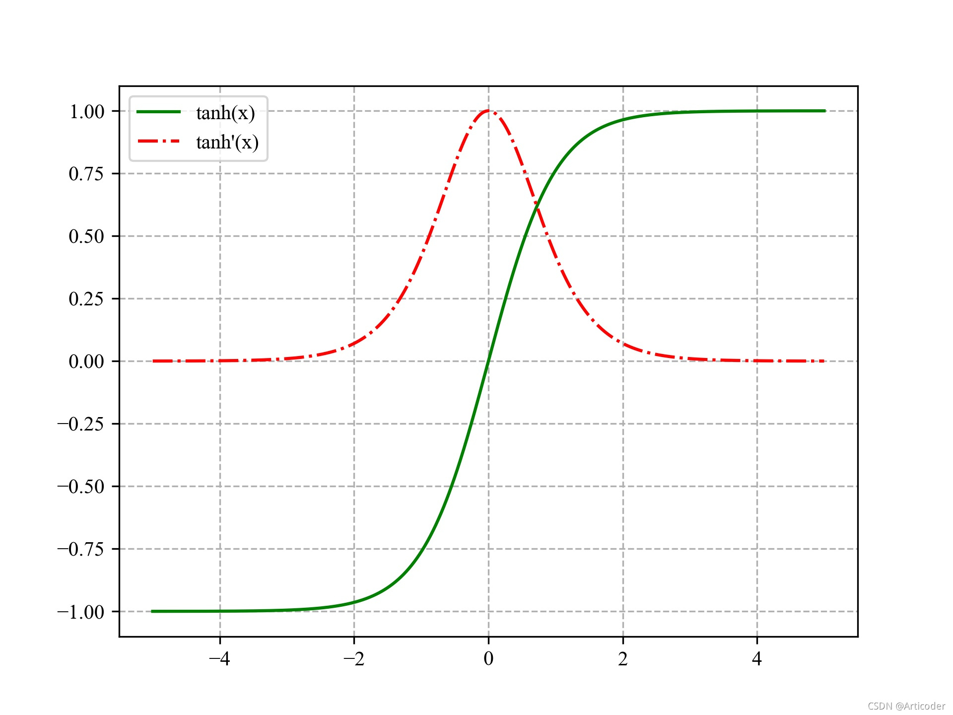
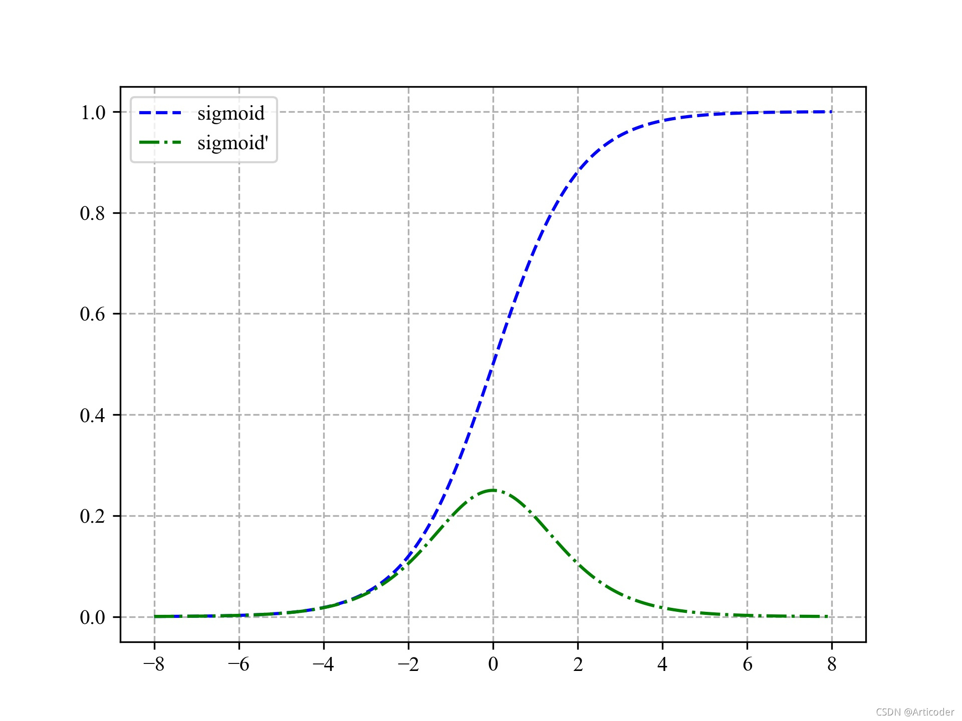
由此可知,不管使用哪种激活函数,其导数的值总不会超过 1 1 1,累乘之后就会出现梯度消失的问题。因此,只有两种解决办法,其一就是使用更好的激活函数(比如 R e L U \rm ReLU ReLU),其二就是改变网络的传播结构,也就是后来提出的 L S T M \rm LSTM LSTM。
长短时记忆网络LSTM
网络结构以及与RNN的区别
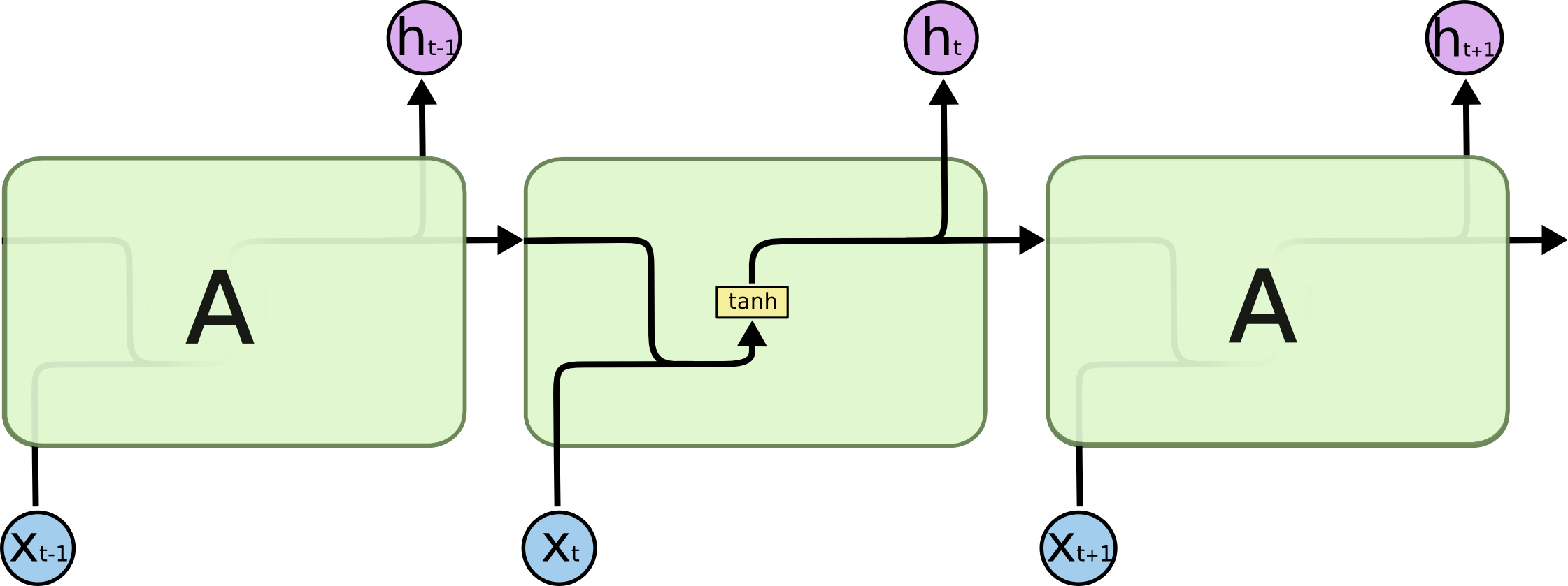
长短时记忆网络 ( L o n g s h o r t − t e r m m e m o r y ) \rm (Long \ short-term \ memory) (Long short−term memory),是一种特殊的循环神经网络,它通过特殊的传播结构设计来避免长期依赖,从而缓解 R N N \rm RNN RNN梯度消失或者爆炸的情形,它在更长的序列中能有更好的表现。 L S T M \rm LSTM LSTM和循环神经网络有基本相同的网络结构,唯一不同的就是单层的前向传播网络模块,单一重复模块有 4 4 4个网络层,以一种特殊的方式进行交互。本质上的不同就是 L S T M \rm LSTM LSTM通过记忆细胞选择性记忆重要信息,过滤掉不重要的信息,减轻记忆负担,而 R N N \rm RNN RNN则记住所有信息,增加了网络的负担。

核心思想
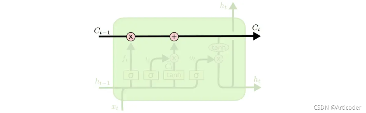
L S T M \rm LSTM LSTM的关键就是细胞状态,也就是下图中的 C t C_t Ct,细胞状态在相当于一个传送带上传送,只有少量的线性交互,所以信息很难流传或者长时间记忆而不发生改变。它主要就是通过称为"门"的结构来控制信号传播以调节细胞状态,从而实现在细胞状态中添加或者删减信息,其中,"门"就是上述结构中的一些相乘或者相加的结构,通过激活函数来使信息选择性通过。
前向传播
遗忘门
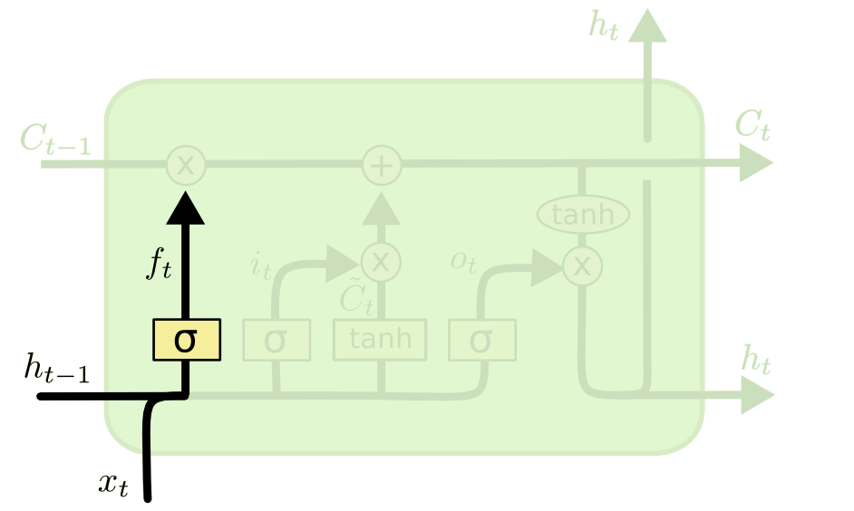
上图所示的是 L S T M \rm LSTM LSTM的第一阶段,也就是"忘记阶段",具体来说,就是通过 h t − 1 h_{t - 1} ht−1和 x t x_t xt计算出 f t ( f o r g e t ) f_t(\rm forget) ft(forget)作为忘记门控,忘记来自细胞状态 C t − 1 C_{t-1} Ct−1中不重要的信息,即对于来此 C t − 1 C_{t-1} Ct−1状态的每个数输出 0 0 0到 1 1 1之间的数, 1 1 1表示完全记住, 0 0 0表示完全忘记。
语言模型的例子中,基于已经看到的预测下一个词。在这个问题中,细胞状态可能包含当前主语的性别,因此正确的代词可以被选择出来。当看到新的主语,希望忘记旧的主语。
f t f_t ft具体计算方式如下
f t = σ ( W x f x t + W h f h t − 1 + b f ) f_t = \sigma(W_{xf} x_t +W_{hf} h_{t - 1} +b_f) ft=σ(Wxfxt+Whfht−1+bf)
输入门

上图所示的是 L S T M \rm LSTM LSTM第二阶段,也就是"输入阶段",就是决定在细胞状态中增加什么信息。其中有两部分,第一部分就是通过 s i g m o i d \rm sigmoid sigmoid函数来确定要添加什么新信息,第二部分就是通过 tanh \tanh tanh函数来创建一个候选值向量 C t ~ \tilde{C_t} Ct~。
具体计算方式如下
i t = σ ( W x i x t + W h i h t − 1 + b i ) C t ~ = tanh ( W x C x t + W h C h t − 1 + b C ) \begin{aligned} i_t &= \sigma(W_{xi}x_t + W_{hi} h_{t-1} +b_i) \\ \tilde{C_t} &= \tanh(W_{xC} x_t + W_{hC} h_{t-1} +b_C) \end{aligned} itCt~=σ(Wxixt+Whiht−1+bi)=tanh(WxCxt+WhCht−1+bC)
状态更新
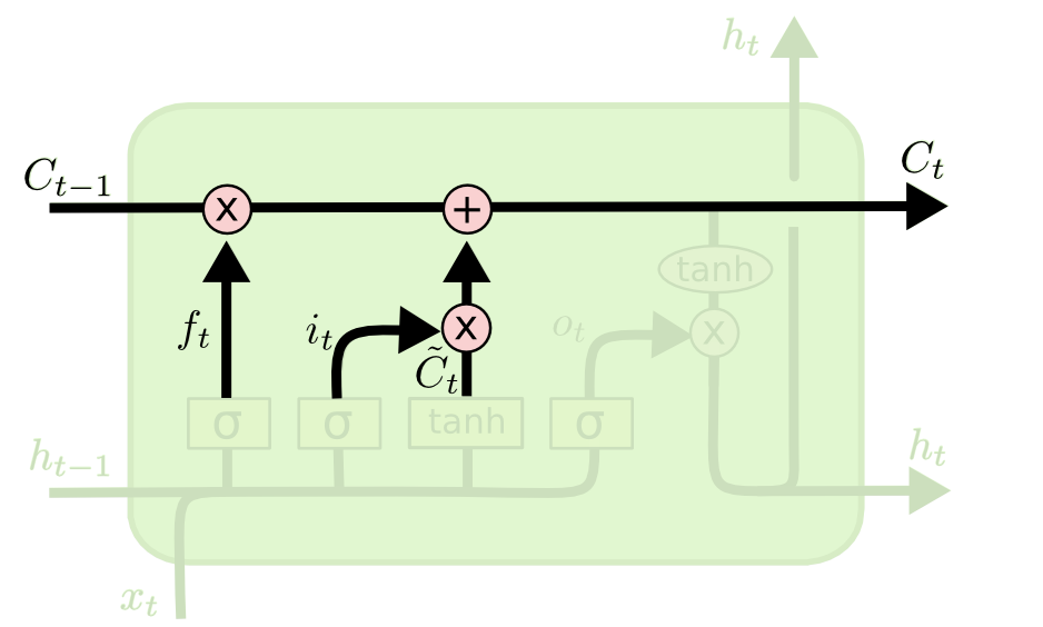
将旧的细胞状态 C t − 1 C_{t - 1} Ct−1更新为 C t C_t Ct,前面的阶段我们已经确定了要遗忘、记住和添加的信息,现在就是实际去完成这个操作。
具体计算方式如下
C t = f t ⊙ C t − 1 + i t ⊙ C t ~ C_t = f_t \odot C_{t-1} + i_t \odot \tilde{C_t} Ct=ft⊙Ct−1+it⊙Ct~
用 f t f_t ft乘以旧的状态 C t − 1 C_{t-1} Ct−1来忘记决定忘记的信息,再加上 i t ⊙ C t ~ i_t \odot \tilde{C_t} it⊙Ct~,它是新的候选值,根据我们决定更新每个状态的程度进行变化。
输出门
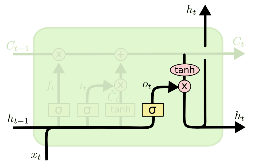
如上图所示,该阶段会决定输出什么值,输出会基于当前细胞状态 C t C_t Ct,也是一个过滤之后的版本。首先通过 s i g m o i d \rm sigmoid sigmoid函数决定当前状态下的哪些输入需要输出,然后将当前细胞状态 C t C_t Ct通过 tanh \tanh tanh函数压缩到 − 1 -1 −1到 1 1 1之间,并将它和 o t o_t ot进行相乘,最终输出我们分。
具体计算方式如下
o t = σ ( W x o x t + W h o h t − 1 + b o ) h t = o t ⊙ tanh ( C t ) \begin{aligned} o_t &= \sigma(W_{xo} x_t + W_{ho} h_{t - 1} + b_o) \\ h_t &= o_t \odot \tanh(C_t) \end{aligned} otht=σ(Wxoxt+Whoht−1+bo)=ot⊙tanh(Ct)
反向传播
首先将前向传播的表达式罗列如下:
{ f t = σ ( W x f x t + W h f h t − 1 + b f ) i t = σ ( W x i x t + W h i h t − 1 + b i ) C ~ t = tanh ( W x C ~ x t + W h C ~ h t − 1 + b C ~ ) C t = f t ⊙ C t − 1 + i t ⊙ C ~ t o t = σ ( W x o x t + W h o h t − 1 + b o ) h t = o t ⊙ tanh ( C t ) y t = W y h t + b y \begin{cases} f_t &= \sigma(W_{xf} x_t +W_{hf}h_{t - 1} +b_f) \\ i_t &= \sigma(W_{xi}x_t + W_{hi} h_{t-1} +b_i) \\ \tilde{C}_t &= \tanh(W_{x\tilde{C}} x_t + W_{h\tilde{C}} h_{t-1} +b_{\tilde{C}}) \\ C_t &= f_t \odot C_{t-1} + i_t \odot \tilde{C}_t \\ o_t &= \sigma(W_{xo} x_t + W_{ho} h_{t - 1} + b_o) \\ h_t &= o_t \odot \tanh(C_t) \\ y_t &= W_y h_t +b_y \end{cases} ⎩⎪⎪⎪⎪⎪⎪⎪⎪⎪⎪⎨⎪⎪⎪⎪⎪⎪⎪⎪⎪⎪⎧ftitC~tCtothtyt=σ(Wxfxt+Whfht−1+bf)=σ(Wxixt+Whiht−1+bi)=tanh(WxC~xt+WhC~ht−1+bC~)=ft⊙Ct−1+it⊙C~t=σ(Wxoxt+Whoht−1+bo)=ot⊙tanh(Ct)=Wyht+by
参数优化
从前向传播的过程中可以看出, 需要优化的参数就只有 W x f , W h f , W x i , W h i , W x C , W h C W x o , W h o , W y W_{xf},W_{hf}, W_{xi},W_{hi}, W_{xC},W_{hC} W_{xo},W_{ho},Wy Wxf,Whf,Wxi,Whi,WxC,WhCWxo,Who,Wy,因此基于它们求导。参照 R N N \rm RNN RNN的反向传播,假设在时刻 t = 3 t= 3 t=3,利用之前时刻的数据对上述优化参数中的 W x f W_{xf} Wxf求
∂ L 3 ∂ W x f ( 3 ) + ∂ L 3 ∂ W x f ( 2 ) + ∂ L 3 ∂ W x f ( 1 ) \frac{\partial{L_3}}{\partial{W_{xf}^{(3)}}} + \frac{\partial{L_3}}{\partial{W_{xf}^{(2)}}} + \frac{\partial{L_3}}{\partial{W_{xf}^{(1)}}} ∂Wxf(3)∂L3+∂Wxf(2)∂L3+∂Wxf(1)∂L3
∂ L 3 ∂ W x f ( 3 ) = ∂ L 3 ∂ y 3 ∂ y 3 ∂ h 3 ∂ h 3 ∂ C 3 ∂ C 3 ∂ f 3 ∂ f 3 ∂ W x f ( 3 ) \frac{\partial{L_3}}{\partial{W_{xf}^{(3)}}} = \frac{\partial{L_3}}{\partial{y_3}} \frac{\partial{y_3}}{\partial{h_3}} \frac{\partial{h_3}}{\partial{C_3}} \frac{\partial{C_3}}{\partial{f_3}} \frac{\partial{f_3}}{\partial{W_{xf}^{(3)}}} \\ ∂Wxf(3)∂L3=∂y3∂L3∂h3∂y3∂C3∂h3∂f3∂C3∂Wxf(3)∂f3
∂ L 3 ∂ W x f ( 2 ) = ∂ L 3 ∂ y 3 ∂ y 3 ∂ h 3 { ∂ h 3 ∂ o 3 ∂ o 3 ∂ h 2 ∂ h 2 ∂ C 2 ∂ h 3 ∂ C 3 { ∂ C 3 ∂ C 2 ∂ C 3 ∂ f 3 ∂ f 3 ∂ h 2 ∂ h 2 ∂ C 2 ∂ C 3 ∂ i 3 ∂ i 3 ∂ h 2 ∂ h 2 ∂ C 2 ∂ C 3 ∂ C ~ 3 ∂ C ~ 3 ∂ h 2 ∂ h 2 ∂ C 2 } } ∂ C 2 ∂ f 2 ∂ f 2 ∂ W x f ( 2 ) = ∂ L 3 ∂ y 3 ∂ y 3 ∂ h 3 { ∂ h 3 ∂ o 3 ∂ o 3 ∂ h 2 ∂ h 2 ∂ C 2 ∂ h 3 ∂ C 3 ∂ C 3 ∂ C 2 } ∂ C 2 ∂ f 2 ∂ f 2 ∂ W x f ( 2 ) \begin{aligned} \frac{\partial{L_3}}{\partial{W_{xf}^{(2)}}} &= \frac{\partial{L_3}}{\partial{y_3}} \frac{\partial{y_3}}{\partial{h_3}} \left\{ \begin{array}{l} \frac{\partial{h_3}}{\partial{o_3}} \frac{\partial{o_3}}{\partial{h_2}} \frac{\partial{h_2}}{\partial{C_2}} \\ \frac{\partial{h_3}}{\partial{C_3}} \left\{ \begin{array}{l} \color{red} { \frac{\partial{C_3}}{\partial{C_2}} }\\ \color{red}{ \frac{\partial{C_3}}{\partial{f_3}} \frac{\partial{f_3}}{\partial{h_2}} \frac{\partial{h_2}}{\partial{C_2}} }\\ \color{red}{ \frac{\partial{C_3}}{\partial{i_3}} \frac{\partial{i_3}}{\partial{h_2}} \frac{\partial{h_2}}{\partial{C_2}} }\\ \color{red}{ \frac{\partial{C_3}}{\partial{\tilde{C}_3}} \frac{\partial{\tilde{C}_3}}{\partial{h_2}} \frac{\partial{h_2}}{\partial{C_2}} } \\ \end{array} \right \} \end{array} \right\} \frac{\partial{C_2}}{\partial{f_2}} \frac{\partial{f_2}}{\partial{W_{xf}^{(2)}}} \\ &= \frac{\partial{L_3}}{\partial{y_3}} \frac{\partial{y_3}}{\partial{h_3}} \left\{ \begin{array}{l} \frac{\partial{h_3}}{\partial{o_3}} \frac{\partial{o_3}}{\partial{h_2}} \frac{\partial{h_2}}{\partial{C_2}} \\ \frac{\partial{h_3}}{\partial{C_3}} \color{red} { \frac{\partial{C_3}}{\partial{C_2}} }\\ \end{array} \right\} \frac{\partial{C_2}}{\partial{f_2}} \frac{\partial{f_2}}{\partial{W_{xf}^{(2)}}} \end{aligned} ∂Wxf(2)∂L3=∂y3∂L3∂h3∂y3⎩⎪⎪⎪⎪⎪⎨⎪⎪⎪⎪⎪⎧∂o3∂h3∂h2∂o3∂C2∂h2∂C3∂h3⎩⎪⎪⎪⎨⎪⎪⎪⎧∂C2∂C3∂f3∂C3∂h2∂f3∂C2∂h2∂i3∂C3∂h2∂i3∂C2∂h2∂C~3∂C3∂h2∂C~3∂C2∂h2⎭⎪⎪⎪⎬⎪⎪⎪⎫⎭⎪⎪⎪⎪⎪⎬⎪⎪⎪⎪⎪⎫∂f2∂C2∂Wxf(2)∂f2=∂y3∂L3∂h3∂y3{
∂o3∂h3∂h2∂o3∂C2∂h2∂C3∂h3∂C2∂C3}∂f2∂C2∂Wxf(2)∂f2
t 3 → t 1 = { t 3 → t 2 : h 3 → { o 3 → h 2 C 3 → C 2 C 3 → f 3 → h 2 C 3 → i 3 → h 2 C 3 → C ~ 3 → h 2 } t 2 → t 1 { C 2 → { f 2 → h 1 → C 1 → f 1 i 2 → h 1 → C 1 → f 1 C ~ 2 → h 1 → C 1 → f 1 C 1 → f 1 } h 2 → { o 2 → h 1 → C 1 → f 1 C 2 → C 1 → f 1 C 2 → f 2 → h 1 → C 1 → f 1 C 2 → i 2 → h 1 → C 1 → f 1 C 2 → C ~ 2 → h 1 → C 1 → f 1 } } } t 3 → t 2 → t 1 : t o t a l 24 p a t h s t_3 \to t_1 = \left\{\begin{array}{l} t_3 \to t_2:h_3 \to \left\{\begin{array}{l} o_3 \to h_2 \\ C_3 \to C_2 \\ C_3 \to f_3 \to h_2 \\ C_3 \to i_3 \to h_2 \\ C_3 \to \tilde{C}_3 \to h_2 \\ \end{array}\right\} \\ t_2 \to t_1 \left\{\begin{array}{l} C_2 \to \left\{\begin{array}{l} f_2 \to h_1 \to C_1 \to f_1 \\ i_2 \to h_1 \to C_1 \to f_1 \\ \tilde{C}_2 \to h_1 \to C_1 \to f_1 \\ C_1 \to f_1 \end{array}\right\} \\ h_2 \to \left\{\begin{array}{l} o_2 \to h_1 \to C_1 \to f_1 \\ C_2 \to C_1 \to f_1 \\ C_2 \to f_2 \to h_1 \to C_1 \to f_1 \\ C_2 \to i_2 \to h_1 \to C_1 \to f_1 \\ C_2 \to \tilde{C}_2 \to h_1 \to C_1 \to f_1 \\ \end{array}\right\} \\ \end{array}\right\} \\ \end{array}\right\} \rm t_3 \to t_2 \to t_1 :total \, 24 \, paths t3→t1=⎩⎪⎪⎪⎪⎪⎪⎪⎪⎪⎪⎪⎪⎪⎪⎪⎪⎪⎪⎪⎪⎪⎪⎨⎪⎪⎪⎪⎪⎪⎪⎪⎪⎪⎪⎪⎪⎪⎪⎪⎪⎪⎪⎪⎪⎪⎧t3→t2:h3→⎩⎪⎪⎪⎪⎨⎪⎪⎪⎪⎧o3→h2C3→C2C3→f3→h2C3→i3→h2C3→C~3→h2⎭⎪⎪⎪⎪⎬⎪⎪⎪⎪⎫t2→t1⎩⎪⎪⎪⎪⎪⎪⎪⎪⎪⎪⎪⎪⎨⎪⎪⎪⎪⎪⎪⎪⎪⎪⎪⎪⎪⎧C2→⎩⎪⎪⎨⎪⎪⎧f2→h1→C1→f1i2→h1→C1→f1C~2→h1→C1→f1C1→f1⎭⎪⎪⎬⎪⎪⎫h2→⎩⎪⎪⎪⎪⎨⎪⎪⎪⎪⎧o2→h1→C1→f1C2→C1→f1C2→f2→h1→C1→f1C2→i2→h1→C1→f1C2→C~2→h1→C1→f1⎭⎪⎪⎪⎪⎬⎪⎪⎪⎪⎫⎭⎪⎪⎪⎪⎪⎪⎪⎪⎪⎪⎪⎪⎬⎪⎪⎪⎪⎪⎪⎪⎪⎪⎪⎪⎪⎫⎭⎪⎪⎪⎪⎪⎪⎪⎪⎪⎪⎪⎪⎪⎪⎪⎪⎪⎪⎪⎪⎪⎪⎬⎪⎪⎪⎪⎪⎪⎪⎪⎪⎪⎪⎪⎪⎪⎪⎪⎪⎪⎪⎪⎪⎪⎫t3→t2→t1:total24paths
∂ L 3 ∂ W x f ( 1 ) = ∂ L 3 ∂ y 3 ∂ y 3 ∂ h 3 { t 3 → t 2 { ∂ h 3 ∂ o 3 ∂ o 3 ∂ h 2 ∂ h 3 ∂ C 3 ∂ C 3 ∂ C 2 ∂ h 3 ∂ C 3 ∂ C 3 ∂ f 3 ∂ f 3 ∂ h 2 ∂ h 3 ∂ C 3 ∂ C 3 ∂ i 3 ∂ i 3 ∂ h 2 ∂ h 3 ∂ C 3 ∂ C 3 ∂ C ~ 3 ∂ C ~ 3 ∂ h 2 } t 2 → t 1 { { ∂ C 2 ∂ f 2 ∂ f 2 ∂ h 1 ∂ h 1 ∂ C 1 ∂ C 2 ∂ i 2 ∂ i 2 ∂ h 1 ∂ h 1 ∂ C 1 ∂ C 2 ∂ C ~ 2 ∂ C ~ 2 ∂ h 1 ∂ h 1 ∂ C 1 ∂ C 2 ∂ C 1 } { ∂ h 2 ∂ o 2 ∂ o 2 ∂ h 1 ∂ h 1 ∂ C 1 ∂ h 2 ∂ C 2 { ∂ C 2 ∂ C 1 ∂ C 2 ∂ f 2 ∂ f 2 ∂ C 1 ∂ C 2 ∂ i 2 ∂ i 2 ∂ h 1 ∂ h 1 ∂ C 1 ∂ C 2 ∂ C ~ 2 ∂ C ~ 2 ∂ h 1 ∂ h 1 ∂ C 1 } } } ∂ C 1 ∂ f 1 } ∂ f 1 ∂ W x f ( 1 ) = ∂ L 3 ∂ y 3 ∂ y 3 ∂ h 3 { t 3 → t 2 { ∂ h 3 ∂ o 3 ∂ o 3 ∂ h 2 ∂ h 3 ∂ C 3 ∂ C 3 ∂ C 2 ∂ h 3 ∂ C 3 ∂ C 3 ∂ f 3 ∂ f 3 ∂ h 2 ∂ h 3 ∂ C 3 ∂ C 3 ∂ i 3 ∂ i 3 ∂ h 2 ∂ h 3 ∂ C 3 ∂ C 3 ∂ C ~ 3 ∂ C ~ 3 ∂ h 2 } t 2 → t 1 { ∂ C 2 ∂ C 1 { ∂ h 2 ∂ o 2 ∂ o 2 ∂ h 1 ∂ h 1 ∂ C 1 ∂ h 2 ∂ C 2 ∂ C 2 ∂ C 1 } } ∂ C 1 ∂ f 1 } ∂ f 1 ∂ W x f ( 1 ) = ∂ L 3 ∂ y 3 ∂ y 3 ∂ h 3 { ∂ h 3 ∂ C 3 ∂ C 3 ∂ C 2 ∂ C 2 ∂ C 1 { ∂ h 3 ∂ o 3 ∂ o 3 ∂ h 2 ∂ h 3 ∂ C 3 ∂ C 3 ∂ f 3 ∂ f 3 ∂ h 2 ∂ h 3 ∂ C 3 ∂ C 3 ∂ i 3 ∂ i 3 ∂ h 2 ∂ h 3 ∂ C 3 ∂ C 3 ∂ C ~ 3 ∂ C ~ 3 ∂ h 2 } ∂ h 2 ∂ o 2 ∂ o 2 ∂ h 1 ∂ h 1 ∂ C 1 ∂ h 3 ∂ o 3 ∂ o 3 ∂ h 2 ∂ h 2 ∂ C 2 ∂ C 2 ∂ C 1 } ∂ C 1 ∂ f 1 ∂ f 1 ∂ W x f ( 1 ) \begin{aligned} \frac{\partial{L_3}}{\partial{W_{xf}^{(1)}}} & = \frac{\partial{L_3}}{\partial{y_3}} \frac{\partial{y_3}}{\partial{h_3}} \left\{\begin{array}{lcl} t_3 \to t_2 \left\{\begin{array}{l} \frac{\partial{h_3}}{\partial{o_3}} \frac{\partial{o_3}}{\partial{h_2}} \\ \frac{\partial{h_3}}{\partial{C_3}} {\color{blue}{ \frac{\partial{C_3}}{\partial{C_2}} }}\\ \frac{\partial{h_3}}{\partial{C_3}} {\color{blue}{ \frac{\partial{C_3}}{\partial{f_3}} \frac{\partial{f_3}}{\partial{h_2}} }}\\ \frac{\partial{h_3}}{\partial{C_3}} {\color{blue}{ \frac{\partial{C_3}}{\partial{i_3}} \frac{\partial{i_3}}{\partial{h_2}} }}\\ \frac{\partial{h_3}}{\partial{C_3}} {\color{blue}{ \frac{\partial{C_3}}{\partial{\tilde{C}_3 }} \frac{\partial{\tilde{C}_3 }}{\partial{h_2}} }}\\ \end{array}\right\} \\ t_2 \to t_1 \left\{\begin{array}{l} \left\{\begin{array}{l} \color{red}{ \frac{\partial{C_2}}{\partial{f_2}} \frac{\partial{f_2}}{\partial{h_1}} \frac{\partial{h_1}}{\partial{C_1}} }\\ \color{red}{ \frac{\partial{C_2}}{\partial{i_2}} \frac{\partial{i_2}}{\partial{h_1}} \frac{\partial{h_1}}{\partial{C_1}} }\\ \color{red}{ \frac{\partial{C_2}}{\partial{\tilde{C}_2}} \frac{\partial{\tilde{C}_2}}{\partial{h_1}} \frac{\partial{h_1}}{\partial{C_1}} }\\ \color{red}{ \frac{\partial{C_2}}{\partial{C_1}} }\\ \end{array}\right\} \\ \left\{\begin{array}{l} \frac{\partial{h_2}}{\partial{o_2}} \frac{\partial{o_2}}{\partial{h_1}} \frac{\partial{h_1}}{\partial{C_1}} \\ {\color{blue}{ \frac{\partial{h_2}}{\partial{C_2}} }} \left\{\begin{array}{l} \color{green}{ \frac{\partial{C_2}}{\partial{C_1}} }\\ \color{green}{ \frac{\partial{C_2}}{\partial{f_2}} \frac{\partial{f_2}}{\partial{C_1}}} \\ \color{green}{ \frac{\partial{C_2}}{\partial{i_2}} \frac{\partial{i_2}}{\partial{h_1}} \frac{\partial{h_1}}{\partial{C_1}} }\\ \color{green}{ \frac{\partial{C_2}}{\partial{\tilde{C}_2}} \frac{\partial{\tilde{C}_2}}{\partial{h_1}} \frac{\partial{h_1}}{\partial{C_1}} }\\ \end{array}\right\} \\ \end{array}\right\} \end{array}\right\} \frac{\partial{C_1}}{\partial{f_1}}\\ \end{array}\right\} \frac{\partial{f_1}}{\partial{W_{xf}^{(1)}}} \\&= \frac{\partial{L_3}}{\partial{y_3}} \frac{\partial{y_3}}{\partial{h_3}} \left\{\begin{array}{l} t_3 \to t_2 \left\{\begin{array}{l} \frac{\partial{h_3}}{\partial{o_3}} \frac{\partial{o_3}}{\partial{h_2}} \\ \frac{\partial{h_3}}{\partial{C_3}} {\color{blue}{ \frac{\partial{C_3}}{\partial{C_2}} }}\\ \frac{\partial{h_3}}{\partial{C_3}} {\color{blue}{ \frac{\partial{C_3}}{\partial{f_3}} \frac{\partial{f_3}}{\partial{h_2}} }}\\ \frac{\partial{h_3}}{\partial{C_3}} {\color{blue}{ \frac{\partial{C_3}}{\partial{i_3}} \frac{\partial{i_3}}{\partial{h_2}} }}\\ \frac{\partial{h_3}}{\partial{C_3}} {\color{blue}{ \frac{\partial{C_3}}{\partial{\tilde{C}_3 }} \frac{\partial{\tilde{C}_3 }}{\partial{h_2}} }}\\ \end{array}\right\} \\ t_2 \to t_1 \left\{\begin{array}{l} {\color{red}{ \frac{\partial{C_2}}{\partial{C_1}}}}\\ \left\{\begin{array}{l} \frac{\partial{h_2}}{\partial{o_2}} \frac{\partial{o_2}}{\partial{h_1}} \frac{\partial{h_1}}{\partial{C_1}} \\ {\color{blue}{ \frac{\partial{h_2}}{\partial{C_2}} }} {\color{green} { \frac{\partial{C_2}}{\partial{C_1}}}} \end{array}\right\} \end{array}\right\} \frac{\partial{C_1}}{\partial{f_1}}\\ \end{array}\right\} \frac{\partial{f_1}}{\partial{W_{xf}^{(1)}}} \\& = \frac{\partial{L_3}}{\partial{y_3}} \frac{\partial{y_3}}{\partial{h_3}} \left\{\begin{array}{l} \frac{\partial{h_3}}{\partial{C_3}} {\color{purple}{ \frac{\partial{C_3}}{\partial{C_2}} }} {\color{red}{ \frac{\partial{C_2}}{\partial{C_1}}}}\\ \left\{\begin{array}{l} \frac{\partial{h_3}}{\partial{o_3}} \frac{\partial{o_3}}{\partial{h_2}} \\ \frac{\partial{h_3}}{\partial{C_3}} {\color{blue}{ \frac{\partial{C_3}}{\partial{f_3}} \frac{\partial{f_3}}{\partial{h_2}} }}\\ \frac{\partial{h_3}}{\partial{C_3}} {\color{blue}{ \frac{\partial{C_3}}{\partial{i_3}} \frac{\partial{i_3}}{\partial{h_2}} }}\\ \frac{\partial{h_3}}{\partial{C_3}} {\color{blue}{ \frac{\partial{C_3}}{\partial{\tilde{C}_3 }} \frac{\partial{\tilde{C}_3 }}{\partial{h_2}} }}\\ \end{array}\right\} \frac{\partial{h_2}}{\partial{o_2}} \frac{\partial{o_2}}{\partial{h_1}} \frac{\partial{h_1}}{\partial{C_1}} \\ \frac{\partial{h_3}}{\partial{o_3}} \frac{\partial{o_3}}{\partial{h_2}} {\color{blue}{ \frac{\partial{h_2}}{\partial{C_2}} }} {\color{green} { \frac{\partial{C_2}}{\partial{C_1}}}}\\ \end{array}\right\} \frac{\partial{C_1}}{\partial{f_1}} \frac{\partial{f_1}}{\partial{W_{xf}^{(1)}}} \end{aligned} ∂Wxf(1)∂L3=∂y3∂L3∂h3∂y3⎩⎪⎪⎪⎪⎪⎪⎪⎪⎪⎪⎪⎪⎪⎪⎪⎪⎪⎪⎪⎪⎪⎪⎪⎪⎪⎪⎪⎨⎪⎪⎪⎪⎪⎪⎪⎪⎪⎪⎪⎪⎪⎪⎪⎪⎪⎪⎪⎪⎪⎪⎪⎪⎪⎪⎪⎧t3→t2⎩⎪⎪⎪⎪⎪⎨⎪⎪⎪⎪⎪⎧∂o3∂h3∂h2∂o3∂C3∂h3∂C2∂C3∂C3∂h3∂f3∂C3∂h2∂f3∂C3∂h3∂i3∂C3∂h2∂i3∂C3∂h3∂C~3∂C3∂h2∂C~3⎭⎪⎪⎪⎪⎪⎬⎪⎪⎪⎪⎪⎫t2→t1⎩⎪⎪⎪⎪⎪⎪⎪⎪⎪⎪⎪⎪⎪⎪⎪⎨⎪⎪⎪⎪⎪⎪⎪⎪⎪⎪⎪⎪⎪⎪⎪⎧⎩⎪⎪⎪⎨⎪⎪⎪⎧∂f2∂C2∂h1∂f2∂C1∂h1∂i2∂C2∂h1∂i2∂C1∂h1∂C~2∂C2∂h1∂C~2∂C1∂h1∂C1∂C2⎭⎪⎪⎪⎬⎪⎪⎪⎫⎩⎪⎪⎪⎪⎪⎨⎪⎪⎪⎪⎪⎧∂o2∂h2∂h1∂o2∂C1∂h1∂C2∂h2⎩⎪⎪⎪⎨⎪⎪⎪⎧∂C1∂C2∂f2∂C2∂C1∂f2∂i2∂C2∂h1∂i2∂C1∂h1∂C~2∂C2∂h1∂C~2∂C1∂h1⎭⎪⎪⎪⎬⎪⎪⎪⎫⎭⎪⎪⎪⎪⎪⎬⎪⎪⎪⎪⎪⎫⎭⎪⎪⎪⎪⎪⎪⎪⎪⎪⎪⎪⎪⎪⎪⎪⎬⎪⎪⎪⎪⎪⎪⎪⎪⎪⎪⎪⎪⎪⎪⎪⎫∂f1∂C1⎭⎪⎪⎪⎪⎪⎪⎪⎪⎪⎪⎪⎪⎪⎪⎪⎪⎪⎪⎪⎪⎪⎪⎪⎪⎪⎪⎪⎬⎪⎪⎪⎪⎪⎪⎪⎪⎪⎪⎪⎪⎪⎪⎪⎪⎪⎪⎪⎪⎪⎪⎪⎪⎪⎪⎪⎫∂Wxf(1)∂f1=∂y3∂L3∂h3∂y3⎩⎪⎪⎪⎪⎪⎪⎪⎪⎪⎪⎪⎪⎪⎨⎪⎪⎪⎪⎪⎪⎪⎪⎪⎪⎪⎪⎪⎧t3→t2⎩⎪⎪⎪⎪⎪⎨⎪⎪⎪⎪⎪⎧∂o3∂h3∂h2∂o3∂C3∂h3∂C2∂C3∂C3∂h3∂f3∂C3∂h2∂f3∂C3∂h3∂i3∂C3∂h2∂i3∂C3∂h3∂C~3∂C3∂h2∂C~3⎭⎪⎪⎪⎪⎪⎬⎪⎪⎪⎪⎪⎫t2→t1⎩⎪⎨⎪⎧∂C1∂C2{ ∂o2∂h2∂h1∂o2∂C1∂h1∂C2∂h2∂C1∂C2}⎭⎪⎬⎪⎫∂f1∂C1⎭⎪⎪⎪⎪⎪⎪⎪⎪⎪⎪⎪⎪⎪⎬⎪⎪⎪⎪⎪⎪⎪⎪⎪⎪⎪⎪⎪⎫∂Wxf(1)∂f1=∂y3∂L3∂h3∂y3⎩⎪⎪⎪⎪⎪⎪⎪⎪⎨⎪⎪⎪⎪⎪⎪⎪⎪⎧∂C3∂h3∂C2∂C3∂C1∂C2⎩⎪⎪⎪⎨⎪⎪⎪⎧∂o3∂h3∂h2∂o3∂C3∂h3∂f3∂C3∂h2∂f3∂C3∂h3∂i3∂C3∂h2∂i3∂C3∂h3∂C~3∂C3∂h2∂C~3⎭⎪⎪⎪⎬⎪⎪⎪⎫∂o2∂h2∂h1∂o2∂C1∂h1∂o3∂h3∂h2∂o3∂C2∂h2∂C1∂C2⎭⎪⎪⎪⎪⎪⎪⎪⎪⎬⎪⎪⎪⎪⎪⎪⎪⎪⎫∂f1∂C1∂Wxf(1)∂f1
从上述计算过程中我们可以看出,在最后的求导结果中,会出现大量如下形式的累乘,
⋯ ∏ t = m n ∂ C t ∂ C t − 1 ⋯ \cdots \prod_{t = m}^{n} \frac{\partial{C_{t}}}{\partial{C_{t-1}}} \cdots ⋯t=m∏n∂Ct−1∂Ct⋯
其中,
∂ C t ∂ C t − 1 = ⊕ { ∂ C t ∂ f t ∂ f t ∂ h t − 1 ∂ h t − 1 ∂ C t − 1 ( = C t − 1 ⋅ W h f σ ′ ⋅ o t − 1 tanh ′ ) ∂ C t ∂ i t ∂ i t ∂ h t − 1 ∂ h t − 1 ∂ C t − 1 ( = C ~ t ⋅ W h i σ ′ ⋅ o t − 1 tanh ′ ) ∂ C t ∂ C ~ t ∂ C ~ t ∂ h t − 1 ∂ h t − 1 ∂ C t − 1 ( = i t ⋅ W h C ~ tanh ′ ⋅ o t − 1 ⋅ tanh ′ ) \frac{\partial{C_{t}}}{\partial{C_{t-1}}} = \oplus\begin{cases} \frac{\partial{C_{t}}}{\partial{f_t}} \frac{\partial{f_{t}}}{\partial{h_{t-1}}} \frac{\partial{h_{t-1}}}{\partial{C_{t-1}}} \left(= C_{t-1} \cdot W_{hf} \sigma' \cdot o_{t-1} \tanh'\right)\\ \frac{\partial{C_{t}}}{\partial{i_t}} \frac{\partial{i_{t}}}{\partial{h_{t-1}}} \frac{\partial{h_{t-1}}}{\partial{C_{t-1}}} \left(= \tilde{C}_{t} \cdot W_{hi}\sigma' \cdot o_{t-1}\tanh'\right)\\ \frac{\partial{C_{t}}}{\partial{\tilde{C}_t}} \frac{\partial{\tilde{C}_{t}}}{\partial{h_{t-1}}} \frac{\partial{h_{t-1}}}{\partial{C_{t-1}}} \left(= i_{t} \cdot W_{h\tilde{C}} \tanh' \cdot o_{t-1} \cdot \tanh'\right)\\ \end{cases} ∂Ct−1∂Ct=⊕⎩⎪⎪⎨⎪⎪⎧∂ft∂Ct∂ht−1∂ft∂Ct−1∂ht−1(=Ct−1⋅Whfσ′⋅ot−1tanh′)∂it∂Ct∂ht−1∂it∂Ct−1∂ht−1(=C~t⋅Whiσ′⋅ot−1tanh′)∂C~t∂Ct∂ht−1∂C~t∂Ct−1∂ht−1(=it⋅WhC~tanh′⋅ot−1⋅tanh′)
通过上式可以看出, ∂ C t ∂ C t − 1 \frac{\partial{C_{t}}}{\partial{C_{t-1}}} ∂Ct−1∂Ct的值可以通过调节参数 W h f , W h i , W h C ~ W_{hf},W_{hi},W_{h\tilde{C}} Whf,Whi,WhC~来灵活控制,为了防止梯度消失,可将其控制在 1 1 1附近,那么就会出现 1 1 1累乘的情况,此处考虑的是 t = 1 , 2 , 3 t=1,2,3 t=1,2,3,当考虑的时刻越多,就会出现越来越多的累乘,除了由上述形式的累乘可以控制之外,其他形式的梯度累乘有可能使梯度消失,因此 ∂ C t ∂ C t − 1 \frac{\partial{C_{t}}}{\partial{C_{t-1}}} ∂Ct−1∂Ct的累乘就大大缓解了梯度消失的问题。
从 L S T M \rm LSTM LSTM的工作机制来解释,就是 t = m t=m t=m到 t = n t=n t=n时刻这一短期时间内,细胞状态中记住的信息基本一致,这样也会使得相邻两时刻的梯度几乎一致,从而缓解梯度消失。
参考资料
[1] B站视频:【重温经典】大白话讲解LSTM长短期记忆网络 如何缓解梯度消失,手把手公式推导反向传播
[2] 人人都能看懂的LSTM介绍及反向传播算法推导(非常详细)
[3] Understanding LSTM Networks
[4] 理解 LSTM 网络