斯坦福cs231n(2017年版)的所有编程作业均采用iPython Notebooks实现,不熟悉的朋友可以提前使用一下Notebooks。编程作业#1主要是手写实现一个kNN分类器来对cifar-10图像数据集进行分类。
目录
1.实验综述

2.导入必要的包
import random  #Python内置的伪随机数模块
import numpy as np
from cs231n.data_utils import load_CIFAR10 #cs231n/data_utils.py
import matplotlib.pyplot as plt

from __future__ import print_function

%matplotlib inline
#该魔法函数使得matplotlib绘图在notebook中显示为内联而不是在新窗口中
#设置绘图的风格
plt.rcParams['figure.figsize'] = (10.0,8.0) #绘图的默认大小
plt.rcParams['image.interpolation'] = 'nearest'
plt.rcParams['image.cmap'] = 'gray'

# notebook将重新加载外部python模块
# 查看 http://stackoverflow.com/questions/1907993/autoreload-of-modules-in-ipython
%load_ext autoreload
%autoreload 2
3.数据集
首先进入项目目录下的cs231n/datasets目录,有一个get_datasets.sh脚本文件:
# Get CIFAR10
wget http://www.cs.toronto.edu/~kriz/cifar-10-python.tar.gz
tar -xzvf cifar-10-python.tar.gz
rm cifar-10-python.tar.gz
该脚本用于下载cifar-10数据集并解压,然后删除压缩包。Mac用户可能会报错,找不到wget命令,此时可以使用Mac包管理工具homebrew,在命令行输入 brew install wget 安装wget即可(如果没有安装homebrew的话自行百度安装)。
在当前目录下,打开命令行,执行该脚本文件./get_datasets.sh,得到解压后的数据集:


- 加载数据集
#加载原始CIFAR-10 数据
cifar10_dir = 'cs231n/datasets/cifar-10-batches-py/'
X_train,y_train,X_test,y_test = load_CIFAR10(cifar10_dir)

#查看训练集和测试集的大小
print("Training data shape: ",X_train.shape)
print("Training labels shape: ",y_train.shape)
print('Test data shape: ', X_test.shape)
print('Test labels shape: ', y_test.shape)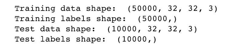
查看#cs231n/data_utils.py 中的load_CIFAR10函数,它用于加载CIFAR-10数据集:
def load_CIFAR10(ROOT):
  """
  加载所有的cifar batch

  input:
  ROOT:解压后cifar数据集的路径

  output:
  Xtr:训练集 四维数组(50000,32,32,3)
  Ytr:训练集图像的标签 一维数组 (50000,)  取值0-9 10个类别
  Xte:测试集 四维数组(10000,32,32,3)
  Yte:测试集图像的标签 一维数组 (10000,) 取值0-9 10个类别
  """

  xs = []  #列表 用于存储cifar训练集 各个batch的数据(四维数组)
  ys = []  #列表 用于存储cifar训练集 各个batch的标签数据(一维数组)
  for b in range(1,6):#b是 batch的编号
    f = os.path.join(ROOT, 'data_batch_%d' % (b, )) #得到各个bacth数据的完整路径
    X, Y = load_CIFAR_batch(f) #得到各个batch中的图片和标签
    xs.append(X) #将每个batch的图片 四维数组 追加到xs中
    ys.append(Y) #将每个batch的图片标签 一维数组 追加到ys中
  Xtr = np.concatenate(xs)  #将列表中所有的四维数组拼接起来  得到完整的训练集图片
  Ytr = np.concatenate(ys)  #将列表中所有的一维数组拼接起来 得到完整的训练集标签
  del X, Y    #删除中间变量X,Y
  Xte, Yte = load_CIFAR_batch(os.path.join(ROOT, 'test_batch')) #得到测试集图片和标签
  return Xtr, Ytr, Xte, Yte
查看load_CIFAR_batch函数:
def load_CIFAR_batch(filename):
  """
  加载cifar一个batch的数据

  input:
  filename:batch的完整路径

  output:
  X:batch中的所有图片 四维数组(10000,32,32,3)
  Y:batch中所有图片标签 一维数组(10000,)
  """
  with open(filename, 'rb') as f: #打开文件 以二进制读取
    datadict = load_pickle(f)  #得到数据字典
    X = datadict['data']     #得到batch中的所有图片
    Y = datadict['labels']   #得到batch中图片的标签
    X = X.reshape(10000, 3, 32, 32).transpose(0,2,3,1).astype("float") #将X转型为(10000,3,32,32)四维数组,并调换一下各个轴  得到(10000,32,32,3)四维数组  数值类型为float(np.float64)
    Y = np.array(Y) #将Y变为一维数组
    return X, Y
查看load_pickle函数:
import platform
from six.moves import cPickle as pickle

def load_pickle(f):
    version = platform.python_version_tuple()#得到Python版本
    if version[0] == '2': #针对Python2
        return  pickle.load(f)
    elif version[0] == '3':  #针对Python3
        return  pickle.load(f, encoding='latin1')
    raise ValueError("invalid python version: {}".format(version))
- 可视化部分样本
#可视化数据集中的一些样本
#展示训练集中不同类别的一些样本图片
classes = ['plane','car','bird','cat','deer','dog','frog','horse','ship','truck']
num_classes = len(classes) #10
samples_per_class = 7 #每个类别取7个样本
for y,cls in enumerate(classes):
    idxs = np.flatnonzero(y_train==y)
    idxs = np.random.choice(idxs, samples_per_class, replace=False)
    for i, idx in enumerate(idxs):
        plt_idx = i * num_classes + y + 1
        plt.subplot(samples_per_class, num_classes, plt_idx)
        plt.imshow(X_train[idx].astype('uint8'))
        plt.axis('off')
        if i == 0:
            plt.title(cls)
plt.show()
- 取部分数据
#取一部分数据 使代码运行更快
#训练集取原始训练集的前5000张
num_training = 5000
mask = list(range(5000))
X_train = X_train[mask]
y_train = y_train[mask]
#测试集取原始测试集的前500张
num_test = 500
mask = list(range(500))
X_test = X_test[mask]
y_test = y_test[mask]- 预处理
#把训练集和测试集张的每张图片32*32*3 拉伸为向量
X_train = X_train.reshape((X_train.shape[0],-1)) #(5000,32*32*3)
X_test = X_test.reshape((X_test.shape[0],-1)) #(500,32*32*3)
print(X_train.shape, X_test.shape)
'''
等价写法
X_train = np.reshape(X_train, (X_train.shape[0], -1))
X_test = np.reshape(X_test, (X_test.shape[0], -1))
'''
3.实现kNN分类器
- 训练kNN
查看kNN类中train方法:
 def train(self, X, y):
    """
    训练KNN分类器,只是记住训练集的数据

    Inputs:
    - X: 训练集样本/图片的特征矩阵,每一行代表一张图片的特征向量,维度(num_train, D)
    - y: 一维数组,包含训练集中每个样本/图片的标签 (num_train,) y[i] 是图片/样本 X[i]的标签.
    """
    self.X_train = X
    self.y_train = y
#导入KNN类
from cs231n.classifiers import KNearestNeighbor
#实例化KNN类的对象
classifier = KNearestNeighbor()
#使用对象调用类中的train方法
#classfier只是简单记住训练集的数据 没有做任何处理
classifier.train(X_train,y_train)- 测试

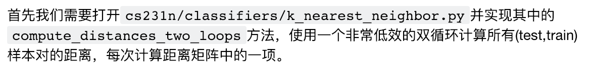
编写类中的计算距离的方法compute_distances_two_loops:
def compute_distances_two_loops(self, X):
    """
    计算测试集X中的每个测试样本和训练集X_train中所有训练样本的距离,使用两个循环遍历所有训练数据和测试数据。

    Inputs:
    - X: 测试集样本的特征矩阵 每一行代表一个样本/图片的特征向量 (num_test, D) .

    Returns:
    - dists: 一个二维数组 (num_test, num_train),(i,j)代表第i个测试样本和第j个训练样本的L2/欧氏距离。
    """

    num_test = X.shape[0] #测试样本/图片数
    num_train = self.X_train.shape[0] #训练样本/图片数
    dists = np.zeros((num_test, num_train)) #初始化距离矩阵
    for i in range(num_test):
      for j in range(num_train):
        dists[i][j] = np.sqrt(np.sum((X[i]-self.X_train[j])**2))

    return dists
#测试实现
#使用kNN类的实例化对象classifier调用类中的方法
dists = classifier.compute_distances_two_loops(X_test)
print(dists.shape)
可视化距离矩阵:
#可视化距离矩阵 每一行代表一个测试样本和所有训练样本的距离
plt.imshow(dists,interpolation='none')
plt.show()
实现类中的predict_labels方法:
def predict_labels(self, dists, k=1):
    """
    给定每个测试样本和所有训练样本的距离矩阵dists,得到每个测试样本的标签。

    Inputs:
    - dists:一个二维数组 (num_test, num_train),(i,j)代表第i个测试样本和第j个训练样本的L2/欧氏距离。

    Returns:
    - y: 一维数组,包含每个测试样本的预测标签,大小 (num_test,)  y[i] 是测试样本 X[i]的预测标签.
    """
    num_test = dists.shape[0] #测试样本的数量
    y_pred = np.zeros(num_test) #初始化y_pred
    for i in range(num_test):
        # closest_y包含与第i个测试样本最近的k个训练样本的标签
        closest_y = []
        closest_y = self.y_train[np.argpartition(dists[i],k)[0:k]]
        #投票 找到这k个训练样本标签中出现次数最多的标签
        y_pred[i] = np.argmax(np.bincount(closest_y))
        '''
        等价写法:
        distances=dists[i,:]
        indexes = np.argsort(distances)
        closest_y=self.y_train[indexes[:k]]
        '''

    return y_pred
#实现cs231n/classifiers/k_nearest_neighbor.py中的predict_labels方法
#测试实现 使用k=1
#使用kNN类的实例化对象classifier调用类中的方法
y_test_pred = classifier.predict_labels(dists,k=1)
#计算预测准确率
num_correct = np.sum(y_test_pred == y_test)
accuracy = float(num_correct)/num_test
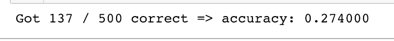
print('Got %d / %d correct => accuracy: %f' % (num_correct, num_test, accuracy))
y_test_pred = classifier.predict_labels(dists, k=5)
num_correct = np.sum(y_test_pred == y_test)
accuracy = float(num_correct) / num_test
print('Got %d / %d correct => accuracy: %f' % (num_correct, num_test, accuracy))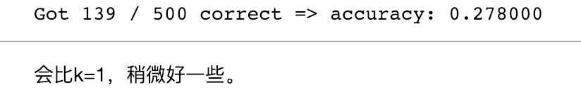
优化距离矩阵的计算方法,编写类中的计算距离的方法compute_distances_one_loops:
def compute_distances_one_loop(self, X):
    """
   计算测试集X中的每个测试样本和训练集X_train中所有训练样本的距离,使用一个循环进行计算,部分向量化

    Input / Output: 和 compute_distances_two_loops相同
    """
    num_test = X.shape[0] #测试样本数
    num_train = self.X_train.shape[0] #训练样本数
    dists = np.zeros((num_test, num_train))#初始化距离矩阵
    for i in range(num_test):
        dists[i,:] = np.sqrt(np.sum((X[i]-self.X_train)**2,axis=1))

    return dists
#现在我们加速距离矩阵的计算,采用部分向量化 只有一个循环
#实现cs231n/classifiers/k_nearest_neighbor.py中的compute_distances_one_loops方法
#使用kNN类的实例化对象classifier调用类中的方法
dists_one = classifier.compute_distances_one_loop(X_test)
#计算两个距离矩阵的相似度 使用Frobenius norm ;两个矩阵的L2距离
difference = np.linalg.norm(dists - dists_one,ord = 'fro')
print('Difference was: %f' % (difference, ))
if difference < 0.001:
print('Good! The distance matrices are the same')
else:
print('Uh-oh! The distance matrices are different')
进一步优化距离矩阵的计算方法,编写类中的计算距离的方法compute_distances_no_loops:
def compute_distances_no_loops(self, X):
    """
    计算测试集X中的每个测试样本和训练集X_train中所有训练样本的距离,不使用任何循环,完全向量化。

    Input / Output: 和compute_distances_two_loops相同
    """
    num_test = X.shape[0]
    num_train = self.X_train.shape[0]
    dists = np.zeros((num_test, num_train))

    te = np.sum(np.square(X),axis=1)
    tr = np.sum(np.square(self.X_train),axis=1)
    M = np.dot(X,self.X_train.T)
    dists = np.sqrt(te.reshape((num_test,1))+tr-2*M) #(500,1)+(5000,) -> (500,5000)+(500,5000) 广播

    return dists
#现在实现计算距离矩阵的完全向量化版本 没有循环
#实现cs231n/classifiers/k_nearest_neighbor.py中的compute_distances_no_loops方法
#使用kNN类的实例化对象classifier调用类中的方法
dists_two = classifier.compute_distances_no_loops(X_test)
#计算矩阵相似度/范数 F范数
difference = np.linalg.norm(dists - dists_two, ord='fro')
print('Difference was: %f' % (difference, ))
if difference < 0.001:
print('Good! The distance matrices are the same')
else:
print('Uh-oh! The distance matrices are different')
比较不同距离矩阵计算方法的速度:
#比较不同实现版本的速度
def time_function(f, *args):
    """
    Call a function f with args and return the time (in seconds) that it took to execute.
    """
    import time
    tic = time.time()
    f(*args)
    toc = time.time()
    return toc - tic

two_loop_time = time_function(classifier.compute_distances_two_loops, X_test)
print('Two loop version took %f seconds' % two_loop_time)

one_loop_time = time_function(classifier.compute_distances_one_loop, X_test)
print('One loop version took %f seconds' % one_loop_time)

no_loop_time = time_function(classifier.compute_distances_no_loops, X_test)
print('No loop version took %f seconds' % no_loop_time)

4.交叉验证

num_folds = 5 #5-交叉验证  把训练集分为5份  任意4份进行训练,一份进行验证
#针对同一个超参数/同一个模型要训练5次
k_choices = [1,3,5,8,10,12,15,20,50,100] #可选择的k值

X_train_folds = []
y_train_folds = []

X_train_folds = np.array_split(X_train,num_folds)
y_train_folds = np.array_split(y_train,num_folds)

k_to_accuracies = {} #用字典存储 不同超参数k下 取得的准确率
for ki in k_choices:  #每个超参数k都有5个准确率 用列表存储
    k_to_accuracies[ki] = []
#交叉验证
for ki in k_choices:
    for fi in range(num_folds):
        X_traini = np.vstack((X_train_folds[0:fi]+X_train_folds[fi+1:]))
        y_traini = np.hstack((y_train_folds[0:fi]+y_train_folds[fi+1:]))

        #实例化KNN类对象
        classifier = KNearestNeighbor()
        #训练
        classifier.train(X_traini,y_traini)

        dists = classifier.compute_distances_no_loops(X_train_folds[fi])

        y_predi = classifier.predict_labels(dists,ki)

        num_correct = np.sum(y_predi==y_train_folds[fi])
        accuracyi = float(num_correct)/len(y_predi)
        k_to_accuracies[ki].append(accuracyi)

for k in sorted(k_to_accuracies):
    for accuracy in k_to_accuracies[k]:
        print('k = %d, accuracy = %f' % (k, accuracy))
绘图:
#绘图
for k in k_choices:
    accuracies = k_to_accuracies[k]
    plt.scatter([k] * len(accuracies), accuracies)

accuracies_mean = np.array([np.mean(v) for k,v in sorted(k_to_accuracies.items())])
accuracies_std = np.array([np.std(v) for k,v in sorted(k_to_accuracies.items())])

plt.errorbar(k_choices, accuracies_mean, yerr=accuracies_std)
plt.title('Cross-validation on k')
plt.xlabel('k')
plt.ylabel('Cross-validation accuracy')
plt.show()
print(accuracies_mean)
print(accuracies_std)
#基于交叉验证的结果,选择一个最好的k值
#然后用这个k值 重新在全部训练集上进行训练  再在测试集上测试
best_k = 1

classifier = KNearestNeighbor()
classifier.train(X_train, y_train)
y_test_pred = classifier.predict(X_test, k=best_k)

# 计算准确率
num_correct = np.sum(y_test_pred == y_test)
accuracy = float(num_correct) / num_test
print('Got %d / %d correct => accuracy: %f' % (num_correct, num_test, accuracy))