				版权声明:如果你觉得写的还可以,可以考虑打赏一下。转载请联系。					https://blog.csdn.net/u011974639/article/details/75363565				</div>
							            <div id="content_views" class="markdown_views">
						<!-- flowchart 箭头图标 勿删 -->
						<svg xmlns="http://www.w3.org/2000/svg" style="display: none;"><path stroke-linecap="round" d="M5,0 0,2.5 5,5z" id="raphael-marker-block" style="-webkit-tap-highlight-color: rgba(0, 0, 0, 0);"></path></svg>
						<p></p><div class="toc">
卷积神经网络简介
卷积神经网络(convolutional neural network,CNN)最初是用来解决图像识别等问题设计的,随着计算机的发展,现在CNN的应用已经非常广泛了,在自然语言处理(NLP)、医药发现、文本处理等等中都有应用。这里我们着重分析CNN在图像处理上的应用。
在早期图像处理识别研究中,最大的问题是如何组织特征,这是因为图像数据不像其他类型的数据可以通过人工理解来提取特征。在图像中,我们很难根据人为理解提取出有效的特征。在深度学习广泛应用之前,我们必须借助SIFT、HoG等特征提取算法结合SVM等机器学习算法进行图像处理识别。
CNN作为一个深度学习架构被提出的最初诉求,是降低对图像数据预处理的要求,以及避免复杂的特征工程。CNN可以直接使用图像作为输入,减少了许多特征提取的手续。CNN的最大特点在于卷积的权值共享结构,大幅度的减少神经网络的参数,同时防治了过拟合。
CNN的提出
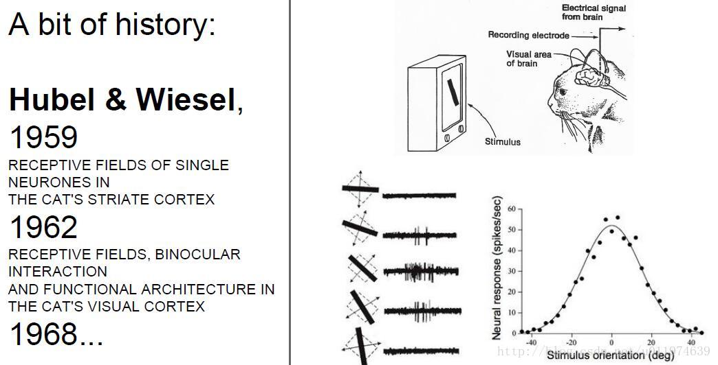
CNN概念最早来自感受野(Receptive Field),科学家对猫的视觉皮层细胞研究发现,每一个视觉神经元只会处理一小块区域的视野图像,即感受野
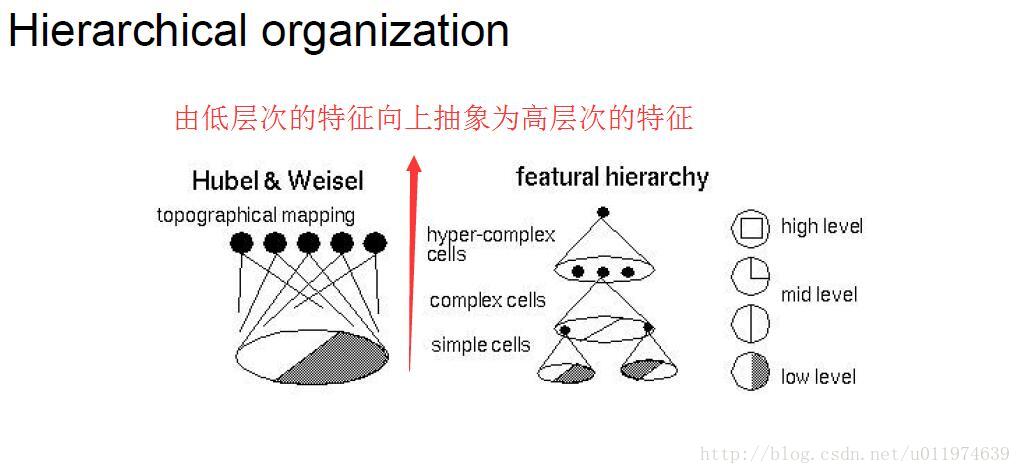
后来,提出神经认识机(Neocognitron)概念,神经认识机包含两类神经元,用来抽取特征的S-cells,还有用来抗形变的C-cells。S-cells对应CNN中的卷积滤波操作,而C-cells则对应激活函数、最大池化等操作。
所以说吧,最厉害的计算机还是大脑.
CNN的壮大
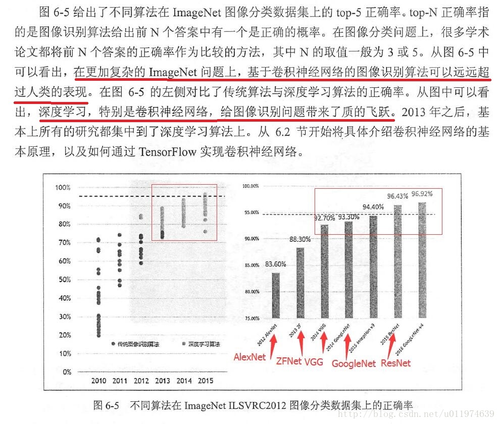
在最近的时间里,CNN最先是在ImageNet上大放光彩,随后被大众熟知,一直到现在成为图像处理的利器。先说说ImageNet.
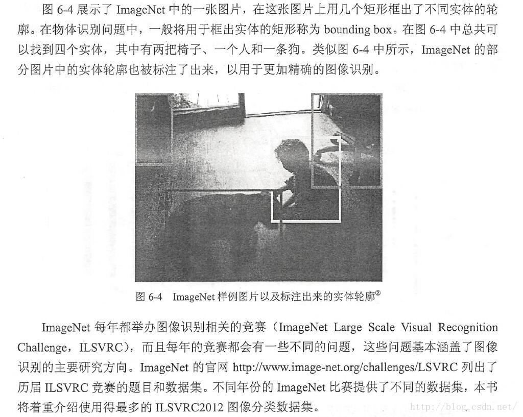
ImageNet是一个基于WordNet(一个大型语义库)的大型图像数据库。在ImageNet中,将近1500万图片被关联到WordNet的大约20000个名词同义词集上,可以被认为是分类问题的一个类别。ImageNet每年都会举办图像识别相关的竞赛(ILSCVRC)。
先总体上对CNN有一个了解,下面该细致的剖析CNN的每个部分
卷积神经网络结构
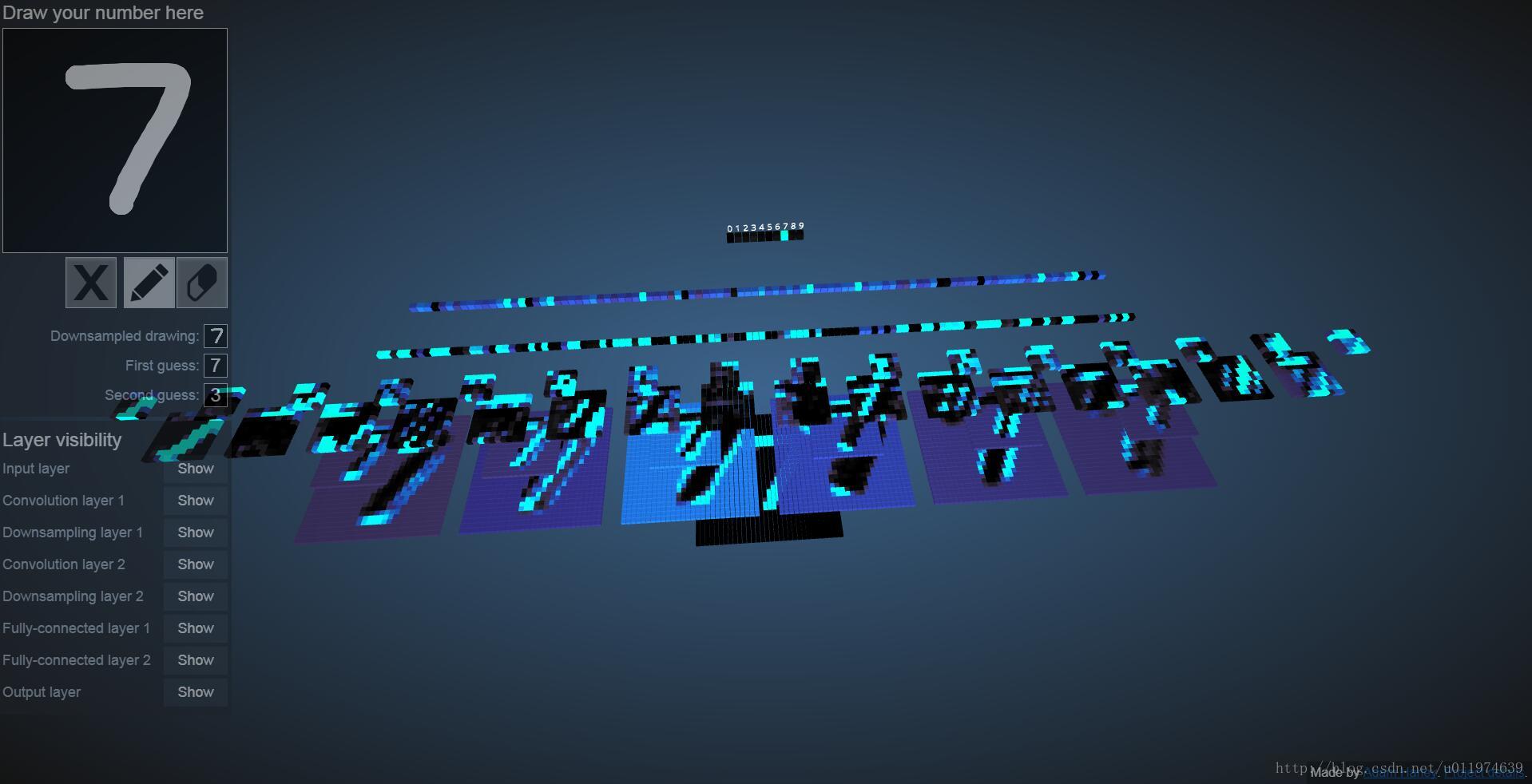
学习CNN的结构之前,可以先到点这里 这个可视化应用上看看CNN的执行流程。
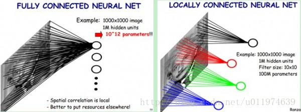
看完后,我们来对比一下CNN与传统神经网络的区别。下图显示了全连接神经网络的结构和CNN的结构对比
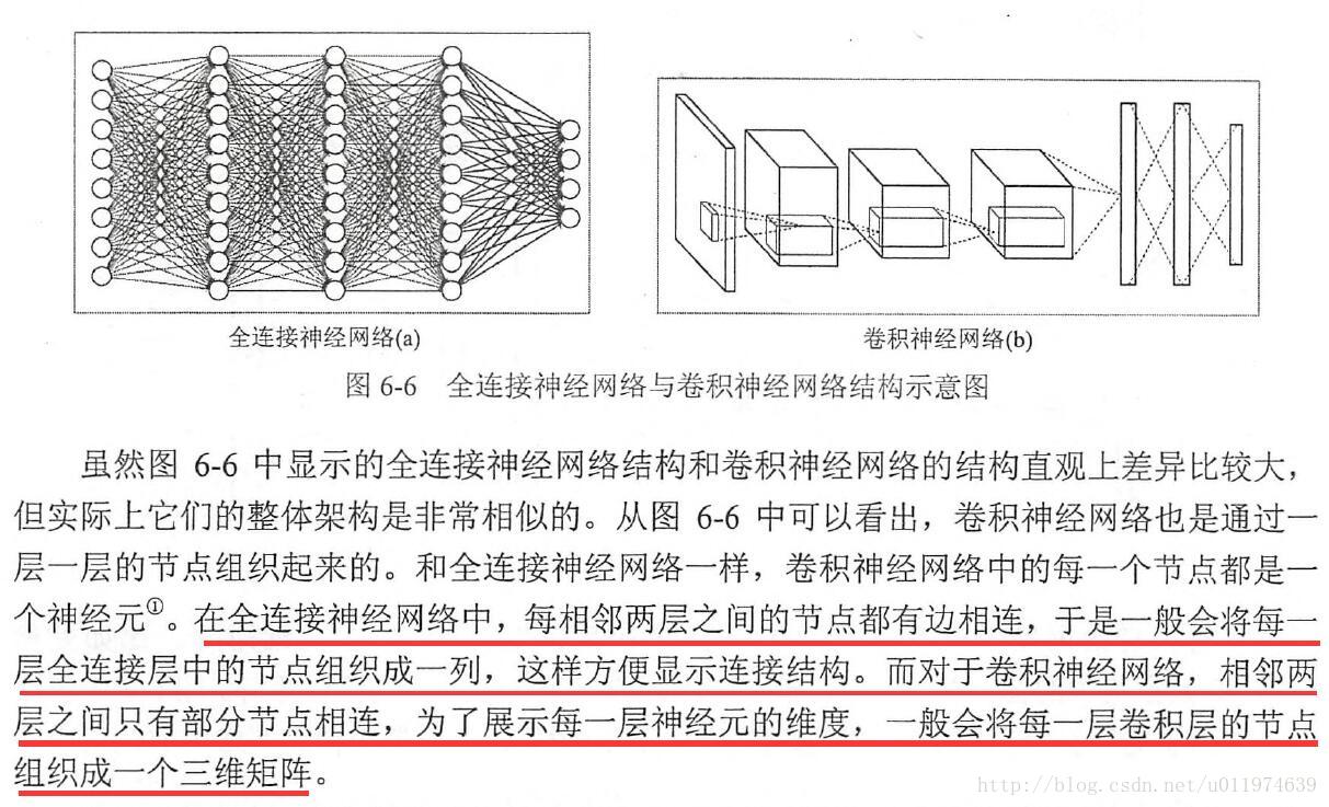
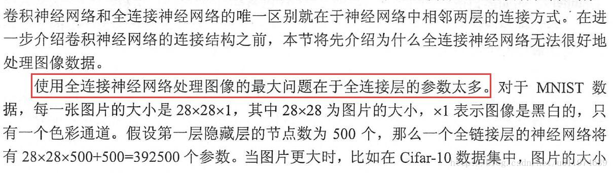
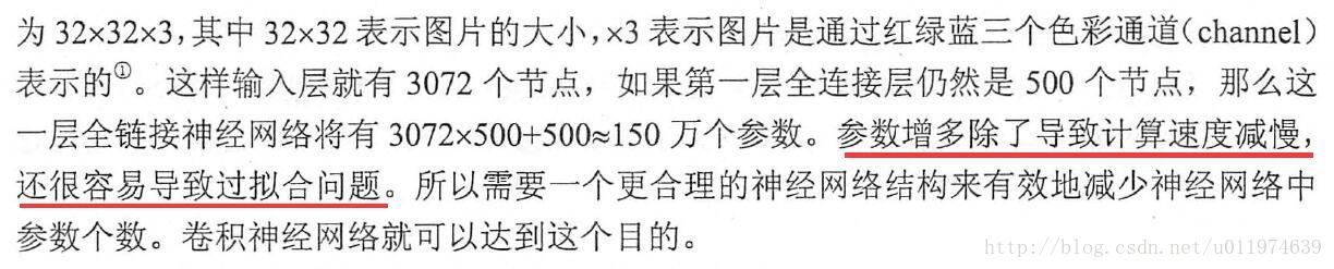
可以看到,CNN相对全连接神经网络所使用的权值参数大大减少了
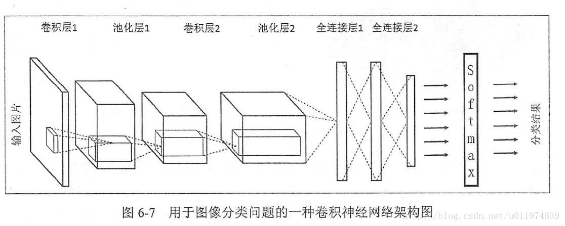
卷积神经网络的常见网络结构
常见的架构图如下:
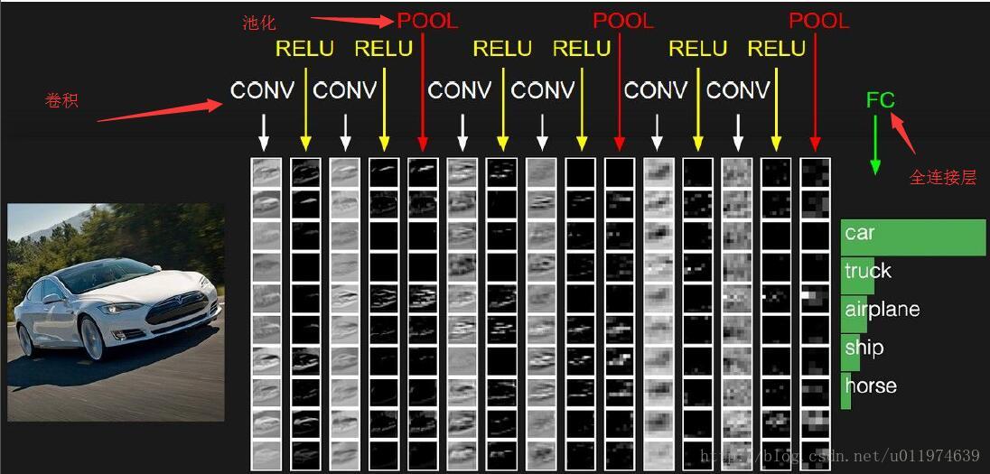
从一个实际的图片类型识别角度来看:
总结下来, 一般来说,一个卷积神经网络主要由以下结构组成:
输入层
输入层是整个神经网络的输入,一般代表的是图片的像素矩阵(一般为三维矩阵,即像素x像素x通道)卷积层
卷积层试图从输入层中抽象出更高的特征。池化层
保留最显著的特征,提升模型的畸变容忍能力。全连接层
图像中被抽象成了信息含量更高的特征在经过神经网络完成后续分类等任务。输出层
一般是使用softmax输出概率值或者分类结果。
在CNN中使用的输入层、输出层、全连接层在前面章节已经介绍过了,下面重点介绍卷积层、池化层。
卷积
再说卷积层之前,我们先谈谈什么的卷积。
信号处理中的卷积
说到卷积,我这个学工科的,最先想到的就是信号处理里面的”线性卷积”、”圆周卷积”,这些怪东西里面的卷积都出自同一个公式。公式如下:
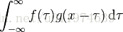
我们可能对这个公式的计算忘得差不多了,但是我们要记得信号处理中的卷积作用:一个函数(f)在另一个函数上(f)的加权叠加。下面我们来对比图像处理中的卷积。
更多卷积的理解可以点这里
图像处理中的卷积
在学习图像处理课程时,接触到了图像卷积。图像处理中的许多操作我们都可以看做是卷积的应用,例如:高斯滤波、均值滤波、膨胀、腐蚀等.
图像处理中的卷积计算,会先定义一个卷积核,而这个卷积核就是定义一个滤波器,卷积核与输入信号做加权叠加得到输出.
也可以理解为二维变量的离散卷积,无论哪种卷积都离不开加权叠加的要义。
图像卷积示例如图:
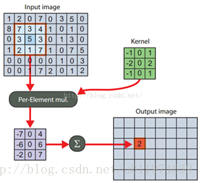
Kernel即定义的卷积核,Kernel与原图像(同等大小的区域)对应的加权叠加得到的值即为输出。
到这里,我们应该对卷积有了一个直观的认识了。
CNN内的卷积层处理和图像处理中的卷积非常相似,下面主要讲讲图像处理中的卷积类型与特点。
卷积的类型的参数
一个常见的卷积过程:
(蓝色为输入数据、阴影为卷积核、绿色为卷积输出)
输入尺寸大小为:4x4
滤波器尺寸大小为:3x3
输出尺寸大小为:2x2
在卷积过程中:有一个步长(stride)参数:步长即每次filter移动的间隔距离。这里stride=1;
如果难以理解stride的含义,看下一个例子。
下图为stride=2(横竖两个方向上)的卷积过程:
输入尺寸大小为:4x4
滤波器尺寸大小为:3x3
输出尺寸大小为:2x2
从上两个例子可以看出,只要滤波器的尺寸不是1x1,那么输出尺寸必定会小于输入尺寸大小,而在实际的图片处理过程中,许多时候我们需要保持图像的大小不变,以便于图像的处理。为了保持输入和输出尺寸一致,同时也有卷积的效果。我们可以对输入图片的外圈做填充操作。
这里我们引入了另外一个参数:padding. zero-padding即在输入的外圈补零的圈数(这里为什么要补零,而不是其他数字:是因为数字零对卷积贡献为零,不会产生额外的偏差).
如果难以理解zero-padding的含义,看下一个例子。
下图为输入图像外圈补一圈零,即padding=1的卷积过程:
输入尺寸大小为:5x5
滤波器尺寸大小为:3x3
输出尺寸大小为:5x5
可以看出输入和输出的尺寸大小一致
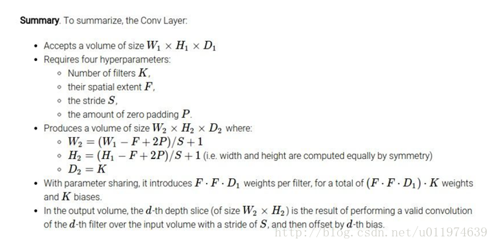
到这里,我们可以给出输入尺寸、输出尺寸、滤波器尺寸、stride和padding的关系:
输入图片的尺寸大小W1 x H1
卷积核(又称滤波器,以下都称滤波器)的大小F x F
输出图片的尺寸大小W2 x H2
stride:S padding:P
关系式如下:
W2 = (W1-F+2P)/S + 1
H2 = (H1-F+2P)/S + 1
除了上述的卷积类型,还有如下的卷积:
更多卷积类型可参考点这里
讲完了各式各样的卷积类型,下面该回归主题,讲讲CNN里面的卷积层了
卷积层
在CNN中,每一个卷积层会直接接受图像像素级输入,每一个卷积操作只会处理一小块图像,经过卷积变换后再传到后面的网络,每一层卷积都会提取数据特征,再经过组合和抽象形成更高阶的特征。
卷积层原理
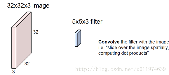
下面剖析一个卷积层的原理:
1.
一张32x32x3的图片(大小为32x32的3通道图片),滤波器大小为5x5x3(滤波器的深度必须与输入层的深度相同).
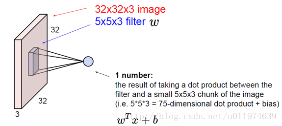
2.
卷积运算同样也是通过向量运算实现的,这里我们把滤波器的值甩成一列向量W.(W大小为75x1).
同时从输入图片中取同样大小的输入数据X(X大小也为75x1),
这样可实现:ωTx+b.(其中b为bias.)这样可实现:ωTx+b.(其中b为bias.)
每一次卷积的输出是一个数值,所以输出层的深度变为1.
- 3.
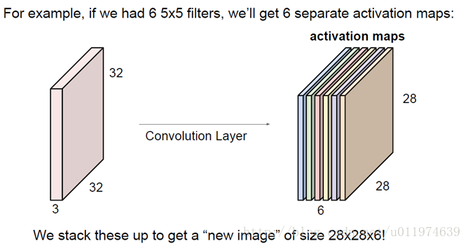
一次完整的卷积过程后,得到一个28x28x1大小的输出图(这里又称为activation maps).
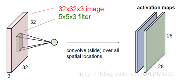
如果我们有6个5x5的滤波器,会得到一个6个28x28x1的输出图,那么叠加到一起就得到28x28x**6**的输出层
- 4.
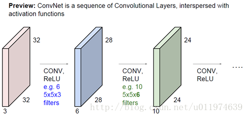
多个卷积层之间连接一起(多层之间又经过了激活函数),从低层的特征抽象到高层的特征.
(这里其实有一个问题:就是多个卷积层直接连接,图像的尺寸会迅速下降,这不是我们想要的,在这里我们可以前面提到的zero-padding来维持输入输出尺寸一致)
实际图片处理过程如下:
到这里,我们讲完的卷积层的运算原理.
卷积层算法
这里我们重点讲解一下输入与输出的尺寸运算,直接引用了cs231n的课件如下:
卷积层特点
一般卷积神经网络由多个卷积层构成,每个卷积层中通常会进行如下几个操作。
- 图像通过多个不同的卷积核的滤波,并添加偏置(bias),提取局部特征,每一个卷积核会映射出一个新的2D图像
- 将前面卷积核的滤波输出结果,进行非线性的激活函数处理
- 对激活函数的结构再进行池化操作(即降采样,后面会详细讲解),目前一般使用最大池化,保留最大特征,提示模型的畸变容忍能力
这几个步骤构成了常见的卷积层,当然也可以再加上LRN(Local Response Normalization,局部响应归一化层),还有Batch Normalization等.
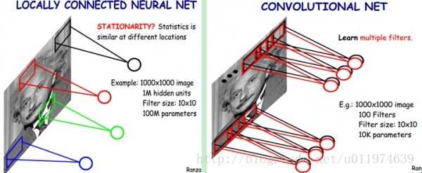
权值共享
每一个卷积层中使用的过滤器参数是相同的,这就是卷积核的权值共享,这是CNN的一个非常重要的性质。
- 从直观上理解,共享卷积核可以使得图像上的内容不受位置的影响,这提高了模型对平移的容忍性,这大大的提高了模型提取特征的能力
- 从网络结构上来说,共享每一个卷积层的卷积核,可以大大减少网络的参数,这不仅可以降低计算的复杂度,而且还能减少因为连接过多导致的严重过拟合,从而提高了模型的泛化能力。
权值共享与传统的全连接的区别如下图:
多卷积核
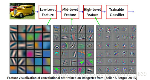
在每一个卷积层中,会使用多个卷积核运算,这是因为每一个卷积核滤波得到的图像就是一类特征的映射,我们提供越多的卷积核,能提供多个方向上的图像特征,可以从图像中抽象出有效而丰富的高阶特征。
池化层
在通过卷积层获得输入的特征时,我们需要做的利用这么特征继续做分类运算。但是针对多个卷积核下的输出特征,依旧会面临着超庞大的参数运算,为了解决这个问题,我们依旧需要减少参数量。这里我们琢磨下,在使用卷积层时,是因为卷积运算可以有效的从输入中提取特征,我们可以对特征做再统计。这一再统计既要能够反映原输入的特征,又要能够降低数据量,我们很自然的想到了取平均值、最大值。这也是池化操作。
池化层原理
从CNN的总体结构上来看,在卷积层之间往往会加入一个池化层(pooling layer).池化层可以非常有效地缩小图片的尺寸。从而减少最后全连接层的参数,在加快计算速度的同时也防止了过拟合的产生。
池化层前向传播过程类似于卷积层的操作一样,也是通过移动一个类似滤波器的结构完成的,不同于卷积层的是,池化层的滤波器计算不是加权求和,而且求区域内的极大值或者平均值。
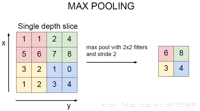
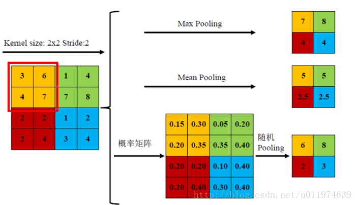
使用最多的是最大值操作的池化层,又称最大池化层(max pooling),计算图像区域内最大值,提取纹理效果较好.
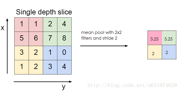
使用平均值操作的池化层,又称平均池化层(mean pooling),计算图像区域的平均值,保留背景更好
随机池化(Stochastic-pooling),介于两者之间,通过对像素点按照数值大小赋予概率,再按照概率进行亚采样
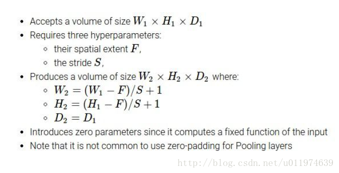
池化层算法
这里我们重点讲解一下输入与输出的尺寸运算,还是引用了cs231n的课件如下:
池化层特点
池化单元的平移不变性
这类似于卷积层的平移不变性。
显著减少参数数量
降采样进一步降低了输出参数量,并赋予模型对轻度形变的容忍性,提高了模型的泛化能力。
到这里,我们算是讲完了CNN的结构了,在回头看看CNN可视化应用,应该会理解的更深吧
TensorFlow中的CNN
说了那么多CNN的理论,下面该看看如何在TensorFlow中实现CNN了
这里按照官方api介绍官方api点这里
卷积
不同的ops下使用的卷积操作总结如下:
- conv2d:Arbitrary filters that can mix channels together(通道混合处理的任意滤波器)
- depthwise_conv2d:Filters that operate on each channel independently.(单独处理每个通道的滤波器)
- separable_conv2d:A depthwise spatial filter followed by a pointwise filter.(一个深度方向的滤波器后跟着一个点滤波器)
strides参数
在TensorFlow中,无论是卷积操作 tf.nn.con2d或者是后面的池化操作tf.nn.max_pool都涉及到了参数strides的指定,这是因为这两种操作都需要在输入图像上滑动滤波器,我们需要指定在每一个维度滑动滤波器的步长.
TensorFlow的文档中给出strides的描述:
A list of ints.一个长度为4的1-D tensor.指定了在输入的Tensor中每个维度滑动滤波的步长。一般要求,strides[0] = strides[3] = 1
为什么要这么要求?
这是因为对于输入而言,无论数据类型是”NHWC”或者”NCHW”,输入的Tensor都包含了[batch,width,height,channels],对应的是strides刚好是这个4个维度的步长。
- 其中strides[0] = 1 代表从batch(即样本)一个一个遍历(如果设置为2,代表间隔性的遍历样本,与其这样,我倒不如缩减样本)
- strides[3] = 1代表在channels上是一个一个通道滑动的(一般我们也是这么做的)
padding参数
根据选择padding的选择为“SAME”或“VALID”的填充方案,计算输出大小和填充像素。
如果为”SAME”,则输出尺寸计算如下:
out_height = ceil(float(in_height) / float(strides[1]))
out_width  = ceil(float(in_width) / float(strides[2]))

在上方和左方填充后计算如下:
pad_along_height = max((out_height - 1) * strides[1] +
            filter_height - in_height, 0)
pad_along_width = max((out_width - 1) * strides[2] +
                   filter_width - in_width, 0)
pad_top = pad_along_height // 2
pad_bottom = pad_along_height - pad_top
pad_left = pad_along_width // 2
pad_right = pad_along_width - pad_left
- 1
- 2
- 3
- 4
- 5
- 6
- 7
- 8
- 9
- 10
- 11
- 12
注意,除以2意味着可能会出现两侧(顶部与底部,右侧和左侧)有多一个填充的情况。 在这种情况下,底部和右侧总是得到一个额外的填充像素。 例如,当pad_along_height为5时,我们在顶部填充2个像素,在底部填充3个像素。 请注意,这不同于现有的库,如cuDNN和Caffe,它们明确指定了填充像素的数量,并且始终在两侧都填充相同数量的像素。
如果为”VALID”,则输出尺寸计算如下:
out_height = ceil(float(in_height - filter_height + 1) / float(strides[1]))
out_width  = ceil(float(in_width - filter_width + 1) / float(strides[2]))

填充值为0,计算输出为:
output[b, i, j, :] =
sum_{di, dj} input[b, strides[1] * i + di - pad_top,
               strides[2] * j + dj - pad_left, ...] *
         filter[di, dj, ...]
- 1
- 2
- 3
- 4
- 5
- 6
- 7
- 8
卷积下常用的方法有:
| 方法(加粗的有详解) | description |
|---|---|
| tf.nn.convolution | Computes sums of N-D convolutions |
| tf.nn.conv2d | Computes a 2-D convolution given 4-D input and filter tensors |
| tf.nn.depthwise_conv2d | Depthwise 2-D convolution |
| tf.nn.depthwise_conv2d_native | Computes a 2-D depthwise convolution given 4-D input and filter tensors. |
| tf.nn.separable_conv2d | Computes a 2-D depthwise convolution given 4-D input and filter tensors |
| tf.nn.atrous_conv2d | 2-D convolution with separable filters |
| tf.nn.atrous_conv2d_transpose | The transpose of atrous_conv2d |
| tf.nn.conv2d_transpose | The transpose of conv2d(卷积的逆向过程) |
| tf.nn.conv1d | Computes a 1-D convolution given 3-D input and filter tensors |
| tf.nn.conv3d | Computes a 3-D convolution given 5-D input and filter tensors |
| tf.nn.conv3d_transpose | The transpose of conv3d |
| tf.nn.conv2d_backprop_filter | Computes the gradients of convolution with respect to the filter. |
| tf.nn.conv2d_backprop_input | Computes the gradients of convolution with respect to the input |
| tf.nn.conv3d_backprop_filter_v2 | Computes the gradients of 3-D convolution with respect to the filter. |
| tf.nn.depthwise_conv2d_native_backprop_filter | Computes the gradients of depthwise convolution with respect to the filter. |
| tf.nn.depthwise_conv2d_native_backprop_input | Computes the gradients of depthwise convolution with respect to the input. |
tf.nn.conv2d
conv2d(
    input,
    filter,
    strides,
    padding,
    use_cudnn_on_gpu=None,
    data_format=None,
    name=None
)
- 1
- 2
- 3
- 4
- 5
- 6
- 7
- 8
- 9
给定输入Tensor的shape为[batch, in_height, in_width, in_channels],滤波器Tensor的shape为 [filter_height, filter_width, in_channels, out_channels], 计算过程如下:
- 将滤波器平坦化为2-D矩阵,形状为[filter_height * filter_width * in_channels,output_channels]
- 从输入张量中提取图像块,形成一个形状为[batch,out_height,out_width,filter_height * filter_width * in_channels]的虚拟张量。
对于每一个图像块,做图像块矢量右乘滤波器矩阵。
#默认格式为NHWC:

output[b, i, j, k] =
sum_{di, dj, q} input[b, strides[1] * i + di, strides[2] * j + dj, q] *
                filter[di, dj, q, k]

必须保持 strides[0] = strides[3] = 1.大多数情况下水平方向和深度方向的步长是一致的:即strides = [1, stride, stride, 1]
- 1
- 2
- 3
- 4
- 5
- 6
- 7
| 参数 | description |
|---|---|
| input | A Tensor.类型必须为如下其一:half, float32 .是一个4-D的Tensor,格式取决于data_format参数 |
| filter | A Tensor.和input类型一致,是一个4-D的Tensor且shape为 [filter_height, filter_width, in_channels, out_channels] |
| strides | A list of ints.一个长度为4的1-D tensor.指定了在输入的Tensor中每个维度滑动滤波的步长 |
| padding | 选择不同的填充方案,可选”SAME”或”VALID” |
| use_cudnn_on_gpu | An optional bool. Defaults to True |
| data_format | 指定输入和输出的数据格式(可选).可选择”NHWC”或者”NCHW”.默认为”NHWC” ”NHWC”:数据按[batch, height, width, channels]存储 ”NCHW”: 数据按[batch, channels, height, width]存储 |
| name | 该ops的name(可选) |
| 返回值 | A Tensor. 类型和input相同,一个4-D的Tensor,格式取决于data_format |
tf.nn.conv3d
conv3d(
    input,
    filter,
    strides,
    padding,
    data_format=None,
    name=None
)
- 1
- 2
- 3
- 4
- 5
- 6
- 7
- 8
在信号处理中,互相关是两个波形的相似度的度量,作为应用于其中之一的时滞的函数。也常被称为 sliding dot product 或sliding inner-product.
我们的Conv3D类似于互相关的处理形式。
| 参数 | description |
|---|---|
| input | A Tensor.类型必须为如下其一:float32,float64,shape为 [batch, in_depth, in_height, in_width, in_channels] |
| filter | A Tensor.和input类型一致.Shape为 [filter_depth, filter_height, filter_width, in_channels, out_channels] in_channels要在input和filter之间匹配 |
| strides | A list of ints.一个长度大于等于5的1-D tensor. 其中要满足strides[0] = strides[4] = 1 |
| padding | 选择不同的填充方案,可选”SAME”或”VALID” |
| data_format | 指定输入和输出的数据格式(可选).可选择”NDHWC”或”NCDHW”.默认为”NDHWC” ”NDHWC”:数据按 [batch, in_depth, in_height, in_width, in_channels]存储 ”NCDHW”: 数据按 [batch, in_channels, in_depth, in_height, in_width]存储 |
| name | 该ops的name(可选) |
| 返回值 | A Tensor. 类型和input相同 |
池化
Each pooling op uses rectangular windows of size ksize separated by offset strides. For example, if strides is all ones every window is used, if strides is all twos every other window is used in each dimension.
In detail, the output is

output[i] = reduce(value[strides * i:strides * i + ksize])
- 1
- 2
- 3
池化常用的方法有:
| 方法(加粗的有详解) | description |
|---|---|
| tf.nn.avg_pool | Performs the average pooling on the input |
| tf.nn.max_pool | Performs the max pooling on the input |
| tf.nn.max_pool_with_argmax | Performs max pooling on the input and outputs both max values and indices |
| tf.nn.avg_pool3d | Performs 3D average pooling on the input |
| tf.nn.max_pool3d | Performs 3D max pooling on the input |
| tf.nn.fractional_avg_pool | Performs fractional average pooling on the input |
| tf.nn.fractional_max_pool | Performs fractional max pooling on the input |
| tf.nn.pool | Performs an N-D pooling operation. |
tf.nn.max_pool
max_pool(
    value,
    ksize,
    strides,
    padding,
    data_format='NHWC',
    name=None
)
- 1
- 2
- 3
- 4
- 5
- 6
- 7
- 8
| 参数 | description |
|---|---|
| value | A 4-D Tensor 类型为 tf.float32. shape为 [batch, height, width, channels] |
| ksize | A list of ints that has length >= 4. The size of the window for each dimension of the input tensor. |
| strides | A list of ints that has length >= 4. The stride of the sliding window for each dimension of the input tensor. |
| padding | ‘VALID’ 或 ‘SAME’ |
| data_format | ‘NHWC’ 或 ‘NCHW’ |
| name | 该ops的name(可选) |
| 返回值 | A Tensor with type tf.float32 |
图形学滤波器
类似于图像处理中的图形学处理(腐蚀、膨胀等)
图形学常用的方法有:
| 方法(加粗的有详解) | description |
|---|---|
| tf.nn.dilation2d(膨胀) | Computes the grayscale dilation of 4-D input and 3-D filter tensors |
| tf.nn.erosion2d(腐蚀) | Computes the grayscale erosion of 4-D value and 3-D kernel tensors |
| tf.nn.with_space_to_batch | Performs op on the space-to-batch representation of input |
激活函数
| 方法(加粗的有详解) | description |
|---|---|
| tf.nn.relu | Computes rectified linear: max(features, 0) |
| tf.nn.relu6 | Computes Rectified Linear 6: min(max(features, 0), 6) |
| tf.nn.crelu | Computes Concatenated ReLU |
| tf.nn.elu | Computes exponential linear: exp(features) - 1 if < 0, features otherwise. |
| tf.nn.softplus | Computes softplus: log(exp(features) + 1). |
| tf.nn.softsign | Computes softsign: features / (abs(features) + 1) |
| tf.nn.dropout | Computes dropout |
| tf.nn.bias_add | Adds bias to value |
| tf.sigmoid | Computes sigmoid of x element-wise |
| tf.tanh | Computes hyperbolic tangent of x element-wise |
tf.nn.relu
relu(
features,
name=None
)
- 1
- 2
- 3
- 4
计算非线性映射:函数关系为 max(features, 0)
| 参数 | description |
|---|---|
| features | A Tensor. 类型是如下一个: float32, float64, int32, int64, uint8, int16, int8, uint16, half |
| name | 该ops的name(可选) |
| 返回值 | A Tensor with sam type as features. |
tf.nn.dropout
dropout(
    x,
    keep_prob,
    noise_shape=None,
    seed=None,
    name=None
)
- 1
- 2
- 3
- 4
- 5
- 6
- 7
使用概率keep_prob,将输入元素按比例放大1 / keep_prob,否则输出0.缩放是为了使预期的和不变
By default, each element is kept or dropped independently. If noise_shape is specified, it must be broadcastable to the shape of x, and only dimensions with noise_shape[i] == shape(x)[i] will make independent decisions. For example, if shape(x) = [k, l, m, n] and noise_shape = [k, 1, 1, n], each batch and channel component will be kept independently and each row and column will be kept or not kept together.
- 1
| 参数 | description |
|---|---|
| x | A tensor. |
| keep_prob | A scalar Tensor with the same type as x. The probability that each element is kept |
| noise_shape | A 1-D Tensor of type int32, representing the shape for randomly generated keep/drop flags |
| seed | A Python integer. Used to create random seeds |
| name | 该ops的name(可选) |
| 返回值 | A Tensor of the same shape of x. |
tf.nn.bias_add
bias_add(
    value,
    bias,
    data_format=None,
    name=None
)
- 1
- 2
- 3
- 4
- 5
- 6
| 参数 | description |
|---|---|
| value | A Tensor with type float, double, int64, int32, uint8, int16, int8, complex64, or complex128. |
| bias | A 1-D Tensor with size matching the last dimension of value. Must be the same type as value unless value is a quantized type, in which case a different quantized type may be used. |
| data_format | ‘NHWC’ or ‘NCHW’ |
| name | 该ops的name(可选) |
| 返回值 | A Tensor with the same type as value |
正则化
| 方法 | description |
|---|---|
| tf.nn.l2_normalize | Normalizes along dimension dim using an L2 norm. |
| tf.nn.local_response_normalization | Local Response Normalization. |
| tf.nn.sufficient_statistics | Calculate the sufficient statistics for the mean and variance of x. |
| tf.nn.normalize_moments | Calculate the mean and variance of based on the sufficient statistics. |
| tf.nn.moments | Calculate the mean and variance of x. |
| tf.nn.weighted_moments | Returns the frequency-weighted mean and variance of x |
| tf.nn.fused_batch_norm | Batch normalization. |
| tf.nn.batch_normalization | Batch normalization. |
| tf.nn.batch_norm_with_global_normalization | Batch normalization. |
损失函数
| 方法(加粗的有详解) | description |
|---|---|
| tf.nn.l2_loss | Computes half the L2 norm of a tensor without the sqrt: output = sum(t ** 2) / 2 |
| tf.nn.log_poisson_loss | Computes log Poisson loss given log_input |
分类器
| 方法(加粗的有详解) | description |
|---|---|
| tf.nn.sigmoid_cross_entropy_with_logits | Computes sigmoid cross entropy given logits |
| tf.nn.softmax | Computes softmax activations |
| tf.nn.log_softmax | Computes log softmax activations: logsoftmax = logits - log(reduce_sum(exp(logits), dim)) |
| tf.nn.softmax_cross_entropy_with_logits | Computes softmax cross entropy between logits and labels |
| tf.nn.sparse_softmax_cross_entropy_with_logits | Computes sparse softmax cross entropy between logits and labels |
| tf.nn.weighted_cross_entropy_with_logits | Computes a weighted cross entropy |
api看完了,该动手撸代码了
TensorFlow实现简易神经网络模型
MNIST数据集下的基础CNN
本节使用的依旧是MNIST数据集,预期可到达到99.1%的准确率。
使用的是结构为卷积–>池化–>卷积–>池化–>全连接层–>softmax层的卷积神经网络。
下面直接贴代码:
    # coding:utf8

    from tensorflow.examples.tutorials.mnist import input_data
    import tensorflow as tf


    def weight_variable(shape):
        '''
        使用卷积神经网络会有很多权重和偏置需要创建,我们可以定义初始化函数便于重复使用
        这里我们给权重制造一些随机噪声避免完全对称,使用截断的正态分布噪声,标准差为0.1
        :param shape: 需要创建的权重Shape
        :return: 权重Tensor
        '''
        initial = tf.truncated_normal(shape, stddev=0.1)
        return tf.Variable(initial)


    def bias_variable(shape):
        '''
        偏置生成函数,因为激活函数使用的是ReLU,我们给偏置增加一些小的正值(0.1)避免死亡节点(dead neurons)
        :param shape:
        :return:
        '''
        initial = tf.constant(0.1, shape=shape)
        return tf.Variable(initial)


    def conv2d(x, W):
        '''
        卷积层接下来要重复使用,tf.nn.conv2d是Tensorflow中的二维卷积函数,
        :param x: 输入 例如[5, 5, 1, 32]代表 卷积核尺寸为5x5,1个通道,32个不同卷积核
        :param W: 卷积的参数
            strides:代表卷积模板移动的步长,都是1代表不遗漏的划过图片的每一个点.
            padding:代表边界处理方式,SAME代表输入输出同尺寸
        :return:
        '''
        return tf.nn.conv2d(x, W, strides=[1, 1, 1, 1], padding="SAME")


    def max_pool_2x2(x):
        '''
        tf.nn.max_pool是TensorFLow中最大池化函数.我们使用2x2最大池化
        因为希望整体上缩小图片尺寸,因而池化层的strides设为横竖两个方向为2步长
        :param x:
        :return:
        '''
        return tf.nn.max_pool(x, ksize=[1, 2, 2, 1], strides=[1, 2, 2, 1], padding="SAME")


    def train(mnist):
        # 使用占位符
        x = tf.placeholder(tf.float32, [None, 784])     # x为特征
        y_ = tf.placeholder(tf.float32, [None, 10])     # y_为label

        # 卷积中将1x784转换为28x28x1  [-1,,,]代表样本数量不变 [,,,1]代表通道数
        x_image = tf.reshape(x, [-1, 28, 28, 1])

        # 第一个卷积层  [5, 5, 1, 32]代表 卷积核尺寸为5x5,1个通道,32个不同卷积核
        # 创建滤波器权值-->加偏置-->卷积-->池化
        W_conv1 = weight_variable([5, 5, 1, 32])
        b_conv1 = bias_variable([32])
        h_conv1 = tf.nn.relu(conv2d(x_image, W_conv1)+b_conv1) #28x28x1 与32个5x5x1滤波器 --> 28x28x32
        h_pool1 = max_pool_2x2(h_conv1)  # 28x28x32 -->14x14x32

        # 第二层卷积层 卷积核依旧是5x5 通道为32   有64个不同的卷积核
        W_conv2 = weight_variable([5, 5, 32, 64])
        b_conv2 = bias_variable([64])
        h_conv2 = tf.nn.relu(conv2d(h_pool1, W_conv2) + b_conv2) #14x14x32 与64个5x5x32滤波器 --> 14x14x64
        h_pool2 = max_pool_2x2(h_conv2)  #14x14x64 --> 7x7x64

        # h_pool2的大小为7x7x64 转为1-D 然后做FC层
        W_fc1 = weight_variable([7*7*64, 1024])
        b_fc1 = bias_variable([1024])
        h_pool2_flat = tf.reshape(h_pool2, [-1, 7*7*64])    #7x7x64 --> 1x3136
        h_fc1 = tf.nn.relu(tf.matmul(h_pool2_flat, W_fc1) + b_fc1)  #FC层传播 3136 --> 1024

        # 使用Dropout层减轻过拟合,通过一个placeholder传入keep_prob比率控制
        # 在训练中,我们随机丢弃一部分节点的数据来减轻过拟合,预测时则保留全部数据追求最佳性能
        keep_prob = tf.placeholder(tf.float32)
        h_fc1_drop = tf.nn.dropout(h_fc1, keep_prob)

        # 将Dropout层的输出连接到一个Softmax层,得到最后的概率输出
        W_fc2 = weight_variable([1024, 10])  #MNIST只有10种输出可能
        b_fc2 = bias_variable([10])
        y_conv = tf.nn.softmax(tf.matmul(h_fc1_drop, W_fc2) + b_fc2)

        # 定义损失函数,依旧使用交叉熵  同时定义优化器  learning rate = 1e-4
        cross_entropy = tf.reduce_mean(-tf.reduce_sum(y_*tf.log(y_conv),reduction_indices=[1]))
        train_step = tf.train.AdamOptimizer(1e-4).minimize(cross_entropy)

        # 定义评测准确率
        correct_prediction = tf.equal(tf.argmax(y_conv, 1), tf.argmax(y_, 1))
        accuracy = tf.reduce_mean(tf.cast(correct_prediction, tf.float32))

        #开始训练
        with tf.Session() as sess:
            init_op = tf.global_variables_initializer() #初始化所有变量
            sess.run(init_op)

            STEPS = 20000
            for i in range(STEPS):
                batch = mnist.train.next_batch(50)
                if i % 100 == 0:
                    train_accuracy = sess.run(accuracy, feed_dict={x: batch[0], y_: batch[1], keep_prob: 1.0})
                    print('step %d,training accuracy %g' % (i, train_accuracy))
                sess.run(train_step, feed_dict={x: batch[0], y_: batch[1], keep_prob: 0.5})

            acc = sess.run(accuracy, feed_dict={x: mnist.test.images, y_: mnist.test.labels, keep_prob: 1.0})
            print("test accuracy %g" % acc)


    if __name__=="__main__":
        mnist = input_data.read_data_sets("MNIST_data/", one_hot=True) # 载入数据集
        train(mnist)
- 1
- 2
- 3
- 4
- 5
- 6
- 7
- 8
- 9
- 10
- 11
- 12
- 13
- 14
- 15
- 16
- 17
- 18
- 19
- 20
- 21
- 22
- 23
- 24
- 25
- 26
- 27
- 28
- 29
- 30
- 31
- 32
- 33
- 34
- 35
- 36
- 37
- 38
- 39
- 40
- 41
- 42
- 43
- 44
- 45
- 46
- 47
- 48
- 49
- 50
- 51
- 52
- 53
- 54
- 55
- 56
- 57
- 58
- 59
- 60
- 61
- 62
- 63
- 64
- 65
- 66
- 67
- 68
- 69
- 70
- 71
- 72
- 73
- 74
- 75
- 76
- 77
- 78
- 79
- 80
- 81
- 82
- 83
- 84
- 85
- 86
- 87
- 88
- 89
- 90
- 91
- 92
- 93
- 94
- 95
- 96
- 97
- 98
- 99
- 100
- 101
- 102
- 103
- 104
- 105
- 106
- 107
- 108
- 109
- 110
- 111
- 112
- 113
- 114
- 115
我配置1080GPU版,训练时间差不多3-4分钟,从4000次开始在训练集上的准确率已经接近为1了,最终在测试集上的准确率差不多为99.3%.
输出:
    Extracting MNIST_data/train-images-idx3-ubyte.gz
    Extracting MNIST_data/train-labels-idx1-ubyte.gz
    Extracting MNIST_data/t10k-images-idx3-ubyte.gz
    Extracting MNIST_data/t10k-labels-idx1-ubyte.gz

    I tensorflow/stream_executor/cuda/cuda_gpu_executor.cc:910] successful NUMA node read from SysFS had negative value (-1), but there must be at least one NUMA node, so returning NUMA node zero
    I tensorflow/core/common_runtime/gpu/gpu_device.cc:885] Found device 0 with properties:
    name: GeForce GTX 1080
    major: 6 minor: 1 memoryClockRate (GHz) 1.873
    pciBusID 0000:01:00.0
    Total memory: 7.92GiB
    Free memory: 6.96GiB
    I tensorflow/core/common_runtime/gpu/gpu_device.cc:906] DMA: 0
    I tensorflow/core/common_runtime/gpu/gpu_device.cc:916] 0:   Y
    I tensorflow/core/common_runtime/gpu/gpu_device.cc:975] Creating TensorFlow device (/gpu:0) -> (device: 0, name: GeForce GTX 1080, pci bus id: 0000:01:00.0)
    step 0,training accuracy 0.06
    step 100,training accuracy 0.84
    step 200,training accuracy 0.92
    step 300,training accuracy 0.88
    step 400,training accuracy 0.98
    step 500,training accuracy 0.96
    step 600,training accuracy 1
    step 700,training accuracy 0.98
    step 800,training accuracy 0.88
    step 900,training accuracy 1
    step 1000,training accuracy 0.94
    step 1100,training accuracy 0.9
    step 1200,training accuracy 1
    step 1300,training accuracy 0.98
    step 1400,training accuracy 0.98
    ....
    step 4200,training accuracy 1
    step 4300,training accuracy 1
    step 4400,training accuracy 1
    step 4500,training accuracy 1
    step 4600,training accuracy 1
    step 4700,training accuracy 0.98
    step 4800,training accuracy 0.96
    step 6700,training accuracy 1
    step 6800,training accuracy 1
    step 6900,training accuracy 1
    ....
    step 19100,training accuracy 1
    step 19200,training accuracy 1
    step 19300,training accuracy 1
    step 19400,training accuracy 1
    step 19500,training accuracy 1
    step 19600,training accuracy 1
    step 19700,training accuracy 1
    step 19800,training accuracy 1
    step 19900,training accuracy 1
    test accuracy 0.993
- 1
- 2
- 3
- 4
- 5
- 6
- 7
- 8
- 9
- 10
- 11
- 12
- 13
- 14
- 15
- 16
- 17
- 18
- 19
- 20
- 21
- 22
- 23
- 24
- 25
- 26
- 27
- 28
- 29
- 30
- 31
- 32
- 33
- 34
- 35
- 36
- 37
- 38
- 39
- 40
- 41
- 42
- 43
- 44
- 45
- 46
- 47
- 48
- 49
- 50
- 51
- 52
可以看到CNN模型的准确率远高于深度神经网络的准确率,这主要归功于CNN的网络设计,CNN对图像特征的提取和抽象能力。依靠这卷积核权值共享,CNN的参数量没有爆炸,训练速度得到保证的同时也减轻了过拟合,整个模型的性能大大提升。
下面是我们使用更为复杂的CNN模型,同时改用CIFAR-10数据集进行测试训练.
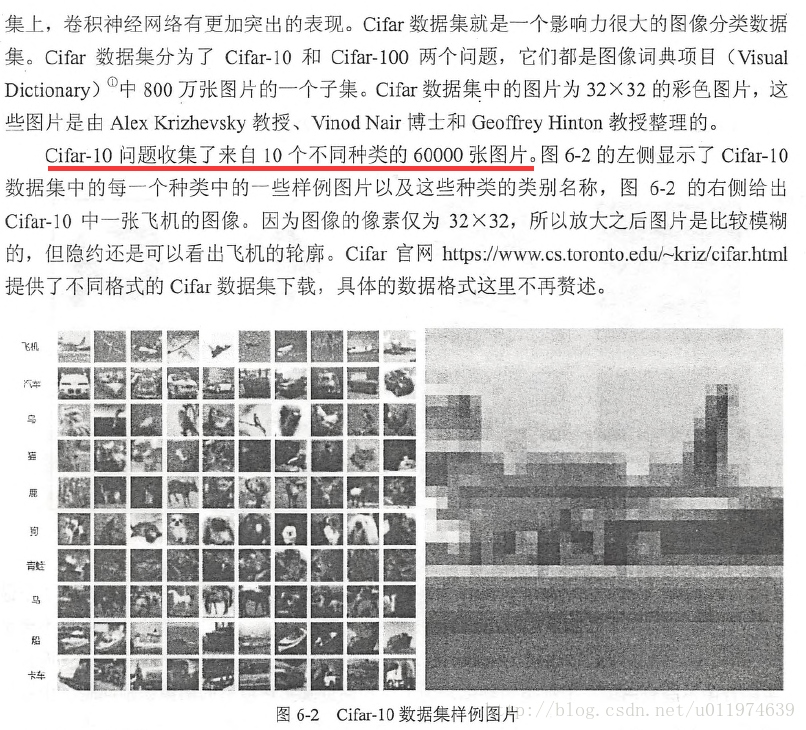
CIFAR-10数据集下的进阶CNN
CIFAR-10数据集介绍
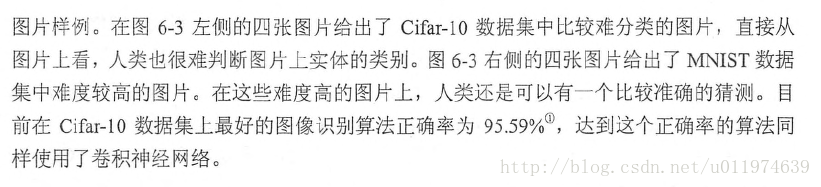
模型修正
- 对weights进行了L2的正则化
- 对输入图片进行翻转、随机剪切等数据增强,制造更多的样本
- 在每个卷积-池化层后使用LRN(局部响应归一化)层,增强模型的泛化能力
本次模型的网络结构如下:
| Layer name | description | shape变化 |
|---|---|---|
| conv1 | 卷积并ReLU激活 | 输入:24x24x3 (filter:64个’SAME’的5x5x3) 输出:24x24x64 |
| pool1 | 最大池化 | 输入:24x24x64 (pool_filter:横竖步长为2的3x3x1) 输出:12x12x64 |
| norm1 | LRN | 输入:12x12x64 输出:12x12x64 |
| conv2 | 卷积并ReLU激活 | 输入:12x12x64 (filter:64个’SAME’的5x5x64) 输出:12x12x64 |
| norm2 | LRN | 输入:12x12x64 输出:12x12x64 |
| pool2 | 最大池化 | 输入:12x12x64 (pool_filter:横竖步长为2的3x3x1) 输出:6x6x64 |
| local3 | FC和ReLU激活 | 输入:6x6x64 (reshape为2304,全连接到下层) 输出:384 |
| local4 | FC和ReLU激活 | 输入:384 (全连接) 输出:192 |
| logits | 计算输出 | 输入:192 (全连接) 输出:10 |
工程实现前的准备
本次我们使用的是cifar10数据集,通常我们会使用tensorflow下封装好的类模块,便于我们使用.
    #从github上下载tensorflow开源项目的测试代码
    #我们使用的是cifar10,进入该目录创建工程(该目录下可以导入cifar10和cifar10-input)
    git clone https://github.com/tensorflow/models
    cd models/tutorials/image/cifar10
- 1
- 2
- 3
- 4
在代码中我们会调用下面函数下载数据集
cifar10.maybe_download_and_extract() #下载数据集并解压
- 1
如果你的电脑在线速度不是很好,可以先加载数据集在点这里cifar10网站下载数据包
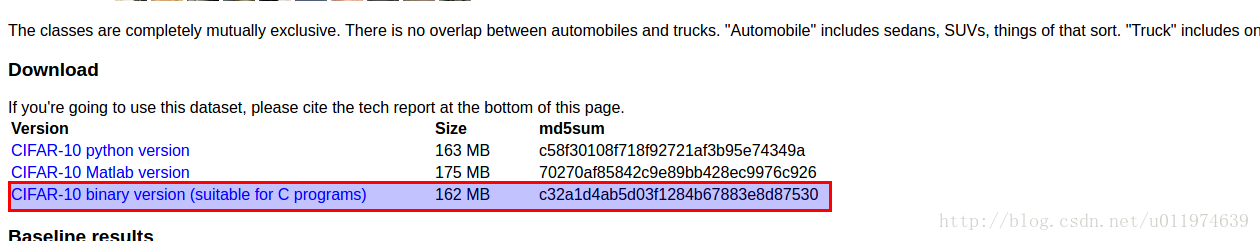
下载完成后,解压到/tmp/cifar10_data目录下,便于后续的数据引用
data_dir = '/tmp/cifar10_data/cifar-10-batches-bin' #代码中引用数据的路径
- 1
准备工作完成后,该开始撸代码了
代码实现
都是老套路了,就直接看代码了
    # coding:utf8

    from __future__ import division
    from models.tutorials.image.cifar10 import cifar10, cifar10_input

    import tensorflow as tf
    import numpy as np
    import time


    def variable_with_weight_loss(shape, stddev, wl):
        '''
        使用tf.truncated_normal截断的正态分布来初始化权重,这里给weight加一个L2的loss.
        我们使用wl控制L2 loss的大小,使用tf.nn.l2_loss计算weight的L2 loss.
        再使用tf.multiply让L2 loss乘wl,得到最后的weight loss,最后将weight loss添加到一个collection.便于后期优化
        :param shape:
        :param stddev:
        :param wl:
        :return:
        '''
        var = tf.Variable(tf.truncated_normal(shape, stddev=stddev))
        if wl is not None:
            weight_loss = tf.multiply(tf.nn.l2_loss(var), wl, name='weight_loss')
            tf.add_to_collection('losses',weight_loss)
        return var


    def loss(logits, labels):
        '''
        使用tf.nn.sparse_softmax_cross_entropy_with_logits将softmax和cross_entropy_loss计算合在一起
        并计算cross_entropy的均值添加到losses集合.以便于后面输出所有losses
        :param logits:
        :param labels:
        :return:
        '''
        labels = tf.cast(labels, tf.int64)
        cross_entropy = tf.nn.sparse_softmax_cross_entropy_with_logits(logits=logits,
                                                            labels=labels, name='cross_entropy_per_example')
        cross_entropy_mean = tf.reduce_mean(cross_entropy, name='cross_entropy')
        tf.add_to_collection('losses',cross_entropy_mean)

        return tf.add_n(tf.get_collection('losses'), name='total_loss')


    def train():
        max_steps = 30000
        batch_size = 128
        data_dir = '/tmp/cifar10_data/cifar-10-batches-bin'

        '''
        使用cifar10_input类中的disorted_inputs函数产生训练数据,产生的数据是已经封装好的Tensor,每次会产生batch_size个
        这个函数已经对图片数据做了增强操作(随机水平翻转/剪切/随机对比度等)
        同时因为对图像处理需要耗费大量计算资源,该函数使用了16个独立的线程来加速任务,
        函数内部会产生线程池,使用会通过TensorFlow queue进行调度
        '''
        images_train,labels_train = cifar10_input.distorted_inputs(data_dir=data_dir, batch_size=batch_size)
        images_test,labels_test = cifar10_input.inputs(eval_data=True, data_dir=data_dir, batch_size=batch_size)

        image_holder = tf.placeholder(tf.float32, [batch_size, 24 ,24, 3])
        label_holder = tf.placeholder(tf.int32, [batch_size])

        # 第一层 卷积-->池化-->lrn
        # 不带L2正则项(wl=0)的64个5x5x3的滤波器,
        # 使用lrn是从局部多个卷积核的响应中挑选比较大的反馈变得相对最大,并抑制其他反馈小的,增加模型泛化能力
        weight1 = variable_with_weight_loss(shape=[5, 5, 3, 64], stddev=5e-2, wl=0.0)
        kernel1 = tf.nn.conv2d(image_holder, weight1, strides=[1, 1, 1, 1], padding='SAME')
        bias1 = tf.Variable(tf.constant(0.0, shape=[64])) #bias直接初始化为0
        conv1 = tf.nn.relu(tf.nn.bias_add(kernel1, bias1))
        pool1 = tf.nn.max_pool(conv1, ksize=[1, 3, 3, 1], strides=[1, 2, 2, 1], padding='SAME')
        norm1 = tf.nn.lrn(pool1, 4, bias=1.0, alpha=0.001/9.0, beta=0.75)

        # 第二层  卷积-->lrn-->池化
        weight2 = variable_with_weight_loss(shape=[5, 5, 64, 64], stddev=5e-2, wl=0.0)
        kernel2 = tf.nn.conv2d(norm1, weight2, strides=[1, 1, 1, 1], padding='SAME')
        bias2 = tf.Variable(tf.constant(0.1,shape=[64]))
        conv2 = tf.nn.relu(tf.nn.bias_add(kernel2, bias2))
        norm2 = tf.nn.lrn(conv2, 4, bias=1.0,alpha=0.001/9.0,beta=0.75)
        pool2 = tf.nn.max_pool(norm2, ksize=[1, 3, 3, 1],strides=[1, 2, 2, 1],padding='SAME')


        #第三层 使用全连接层 reshape后获取长度并创建FC1层的权重(带L2正则化)
        reshape = tf.reshape(pool2, [batch_size, -1])
        dim = reshape.get_shape()[1].value
        weight3 = variable_with_weight_loss(shape=[dim, 384], stddev=0.04, wl=0.004)
        bias3 = tf.Variable(tf.constant(0.1,shape=[384]))
        local3 = tf.nn.relu(tf.matmul(reshape, weight3) + bias3)

        #第四层 FC2层  节点数减半  依旧带L2正则
        weight4 = variable_with_weight_loss(shape=[384, 192], stddev=0.04, wl=0.004)
        bias4 = tf.Variable(tf.constant(0.1, shape=[192]))
        local4 = tf.nn.relu(tf.matmul(local3,weight4) + bias4)

        #最后一层 这层的weight设为正态分布标准差设为上一个FC层的节点数的倒数
        #这里我们不计算softmax,把softmax放到后面计算
        weight5 = variable_with_weight_loss(shape=[192,10], stddev=1/192.0, wl=0.0)
        bias5 = tf.Variable(tf.constant(0.0, shape=[10]))
        logits = tf.add(tf.matmul(local4, weight5),bias5)

        #损失函数为两个带L2正则的FC层和最后的转换层
        #优化器依旧是AdamOptimizer,学习率是1e-3
        losses = loss(logits, label_holder)
        train_op = tf.train.AdamOptimizer(1e-3).minimize(losses)

        #in_top_k函数求出输出结果中top k的准确率,这里选择输出top1
        top_k_op = tf.nn.in_top_k(logits, label_holder, 1)

        #创建默认session,初始化变量
        sess = tf.InteractiveSession()
        tf.global_variables_initializer().run()

        #启动图片增强线程队列
        tf.train.start_queue_runners()

        #训练
        for step in range(max_steps):
            start_time = time.time()
            image_batch,label_batch = sess.run([images_train, labels_train])
            _,loss_value = sess.run([train_op, losses], feed_dict={image_holder: image_batch,
                                                                label_holder: label_batch})
            duration = time.time() - start_time

            if step % 10 == 0:
                examples_per_sec = batch_size / duration
                sec_per_batch = float(duration)

                format_str = ('step %d,loss=%.2f (%.1f examples/sec; %.3f sec/batch)')
                print(format_str % (step, loss_value, examples_per_sec, sec_per_batch))

        #评估模型的准确率,测试集一共有10000个样本
        #我们先计算大概要多少个batch能测试完所有样本
        num_examples = 10000
        import math
        num_iter = int(math.ceil(num_examples / batch_size))
        true_count = 0
        total_sample_count = num_iter * batch_size  #除去不够一个batch的
        step = 0
        while step < num_iter:
            image_batch, label_batch = sess.run([images_test, labels_test])
            predictions = sess.run([top_k_op], feed_dict={image_holder: image_batch,
                                                          label_holder: label_batch})
            true_count += np.sum(predictions)  #利用top_k_op计算输出结果
            step += 1

        precision = true_count / total_sample_count
        print('precision @ 1=%.3f' % precision)  #这里如果输出为0.00 是因为整数/整数  记得要导入float除法


    if __name__ == '__main__':
        cifar10.maybe_download_and_extract()
        train()
- 1
- 2
- 3
- 4
- 5
- 6
- 7
- 8
- 9
- 10
- 11
- 12
- 13
- 14
- 15
- 16
- 17
- 18
- 19
- 20
- 21
- 22
- 23
- 24
- 25
- 26
- 27
- 28
- 29
- 30
- 31
- 32
- 33
- 34
- 35
- 36
- 37
- 38
- 39
- 40
- 41
- 42
- 43
- 44
- 45
- 46
- 47
- 48
- 49
- 50
- 51
- 52
- 53
- 54
- 55
- 56
- 57
- 58
- 59
- 60
- 61
- 62
- 63
- 64
- 65
- 66
- 67
- 68
- 69
- 70
- 71
- 72
- 73
- 74
- 75
- 76
- 77
- 78
- 79
- 80
- 81
- 82
- 83
- 84
- 85
- 86
- 87
- 88
- 89
- 90
- 91
- 92
- 93
- 94
- 95
- 96
- 97
- 98
- 99
- 100
- 101
- 102
- 103
- 104
- 105
- 106
- 107
- 108
- 109
- 110
- 111
- 112
- 113
- 114
- 115
- 116
- 117
- 118
- 119
- 120
- 121
- 122
- 123
- 124
- 125
- 126
- 127
- 128
- 129
- 130
- 131
- 132
- 133
- 134
- 135
- 136
- 137
- 138
- 139
- 140
- 141
- 142
- 143
- 144
- 145
- 146
- 147
- 148
- 149
- 150
输出:
一共训练了30000轮,最后准确率能达到79.4%
    step 0,loss=4.67 (6.6 examples/sec; 19.420 sec/batch)
    step 10,loss=3.64 (2547.1 examples/sec; 0.050 sec/batch)
    step 20,loss=3.27 (2463.0 examples/sec; 0.052 sec/batch)
    step 30,loss=2.75 (2624.5 examples/sec; 0.049 sec/batch)
    step 40,loss=2.43 (2582.4 examples/sec; 0.050 sec/batch)
    step 50,loss=2.31 (2464.1 examples/sec; 0.052 sec/batch)
    step 60,loss=2.20 (2585.5 examples/sec; 0.050 sec/batch)
    step 70,loss=1.98 (2622.6 examples/sec; 0.049 sec/batch)
    step 80,loss=2.05 (2560.3 examples/sec; 0.050 sec/batch)
    step 90,loss=2.06 (2482.5 examples/sec; 0.052 sec/batch)
    step 100,loss=1.96 (2544.2 examples/sec; 0.050 sec/batch)
    step 110,loss=1.83 (2432.1 examples/sec; 0.053 sec/batch)
    ....
    step 29920,loss=0.69 (2439.3 examples/sec; 0.052 sec/batch)
    step 29930,loss=0.71 (2563.3 examples/sec; 0.050 sec/batch)
    step 29940,loss=0.80 (2488.2 examples/sec; 0.051 sec/batch)
    step 29950,loss=0.83 (2564.5 examples/sec; 0.050 sec/batch)
    step 29960,loss=0.80 (2643.3 examples/sec; 0.048 sec/batch)
    step 29970,loss=0.75 (2488.7 examples/sec; 0.051 sec/batch)
    step 29980,loss=0.66 (2516.7 examples/sec; 0.051 sec/batch)
    step 29990,loss=0.77 (2464.1 examples/sec; 0.052 sec/batch)
    precision @ 1=0.794
- 1
- 2
- 3
- 4
- 5
- 6
- 7
- 8
- 9
- 10
- 11
- 12
- 13
- 14
- 15
- 16
- 17
- 18
- 19
- 20
- 21
- 22
过增加max_steps可以增加模型的准确率,如果max_steps很大,可以使用带衰减的learning rate.
总结
在训练前,我们调用了cifar10_input.distorted_inputs实现了样本的数据增强,它可以给单幅图增加多个副本,提高图片的利用率,防止对某一张图片学习过拟合。这也恰恰是利用图片本身的信息,图片的冗余信息量比较大,我们可以制造不同的噪声并让图片依然可以很好的识别出来,这样模型的泛化能力必然会增强。
从本节的例子来看,卷积层一般需要和一个池化层连接,这已经是图像处理里面的标准组件了,在实现中,我们还有添加lrn/l2正则化/权值初始化等Trick.怎样才能搭建一个好的模型,这需要在大量的实践和学习中摸索
本节重点讲解了CNN的概念原理,简单的实现了下CNN网络.下一节我们学习CNN里几个经典的模型,动手搭建一下
参考资料
Stanford University CS231n学习课程 http://cs231n.stanford.edu/
《TensorFlow实战Google深度学习框架》 - 才云科技 郑泽宇等
《TensorFlow实战》 -黄文坚等
卷积的理解:https://www.zhihu.com/question/22298352
卷积动态图:http://blog.csdn.net/liyuan123zhouhui/article/details/60139790
深入浅出池化层(pooling):https://zhuanlan.zhihu.com/p/26069150
TensorFlow官方api:https://www.tensorflow.org/api_guides/python
				<script>
					(function(){
						function setArticleH(btnReadmore,posi){
							var winH = $(window).height();
							var articleBox = $("div.article_content");
							var artH = articleBox.height();
							if(artH > winH*posi){
								articleBox.css({
									'height':winH*posi+'px',
									'overflow':'hidden'
								})
								btnReadmore.click(function(){
									if(typeof window.localStorage === "object" && typeof window.csdn.anonymousUserLimit === "object"){
										if(!window.csdn.anonymousUserLimit.judgment()){
											window.csdn.anonymousUserLimit.Jumplogin();
											return false;
										}else if(!currentUserName){
											window.csdn.anonymousUserLimit.updata();
										}
									}

									articleBox.removeAttr("style");
									$(this).parent().remove();
								})
							}else{
								btnReadmore.parent().remove();
							}
						}
						var btnReadmore = $("#btn-readmore");
						if(btnReadmore.length>0){
							if(currentUserName){
								setArticleH(btnReadmore,3);
							}else{
								setArticleH(btnReadmore,1.2);
							}
						}
					})()
				</script>
				</article>
				版权声明:如果你觉得写的还可以,可以考虑打赏一下。转载请联系。					https://blog.csdn.net/u011974639/article/details/75363565				</div>
							            <div id="content_views" class="markdown_views">
						<!-- flowchart 箭头图标 勿删 -->
						<svg xmlns="http://www.w3.org/2000/svg" style="display: none;"><path stroke-linecap="round" d="M5,0 0,2.5 5,5z" id="raphael-marker-block" style="-webkit-tap-highlight-color: rgba(0, 0, 0, 0);"></path></svg>
						<p></p><div class="toc">