分享一下我老师大神的人工智能教程!零基础,通俗易懂!http://blog.csdn.net/jiangjunshow
也欢迎大家转载本篇文章。分享知识,造福人民,实现我们中华民族伟大复兴!
DeepLearning tutorial(4)CNN卷积神经网络原理简介+代码详解
@author:wepon
@blog:http://blog.csdn.net/u012162613/article/details/43225445
本文介绍多层感知机算法,特别是详细解读其代码实现,基于python theano,代码来自:Convolutional Neural Networks (LeNet)。经详细注释的代码和原始代码:放在我的github地址上,可下载。
一、CNN卷积神经网络原理简介
要讲明白卷积神经网络,估计得长篇大论,网上有很多博文已经写得很好了,所以本文就不重复了,如果你了解CNN,那可以往下看,本文主要是详细地解读CNN的实现代码。如果你没学习过CNN,在此推荐周晓艺师兄的博文:Deep Learning(深度学习)学习笔记整理系列之(七),以及UFLDL上的卷积特征提取、池化
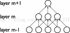
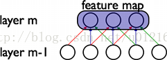
CNN的最大特点就是稀疏连接(局部感受)和权值共享,如下面两图所示,左为稀疏连接,右为权值共享。稀疏连接和权值共享可以减少所要训练的参数,减少计算复杂度。
至于CNN的结构,以经典的LeNet5来说明:
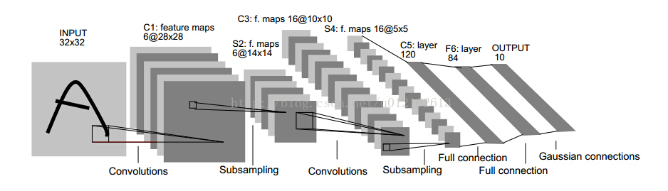
这个图真是无处不在,一谈CNN,必说LeNet5,这图来自于这篇论文:Gradient-Based Learning Applied to Document Recognition,论文很长,第7页那里开始讲LeNet5这个结构,建议看看那部分。
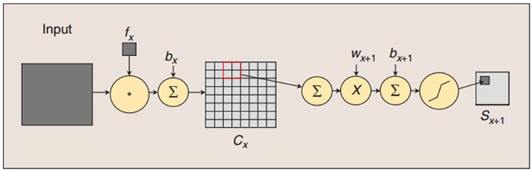
我这里简单说一下,LeNet5这张图从左到右,先是input,这是输入层,即输入的图片。input-layer到C1这部分就是一个卷积层(convolution运算),C1到S2是一个子采样层(pooling运算),关于卷积和子采样的具体过程可以参考下图:
然后,S2到C3又是卷积,C3到S4又是子采样,可以发现,卷积和子采样都是成对出现的,卷积后面一般跟着子采样。S4到C5之间是全连接的,这就相当于一个MLP的隐含层了(如果你不清楚MLP,参考《DeepLearning tutorial(3)MLP多层感知机原理简介+代码详解》)。C5到F6同样是全连接,也是相当于一个MLP的隐含层。最后从F6到输出output,其实就是一个分类器,这一层就叫分类层。
ok,CNN的基本结构大概就是这样,由输入、卷积层、子采样层、全连接层、分类层、输出这些基本“构件”组成,一般根据具体的应用或者问题,去确定要多少卷积层和子采样层、采用什么分类器。当确定好了结构以后,如何求解层与层之间的连接参数?一般采用向前传播(FP)+向后传播(BP)的方法来训练。具体可参考上面给出的链接。
二、CNN卷积神经网络代码详细解读(基于python+theano)
- 没有实现location-specific gain and bias parameters
- 用的是maxpooling,而不是average_pooling
- 分类器用的是softmax,LeNet5用的是rbf
- LeNet5第二层并不是全连接的,本程序实现的是全连接
另外,代码里将卷积层和子采用层合在一起,定义为“LeNetConvPoolLayer“(卷积采样层),这好理解,因为它们总是成对出现。但是有个地方需要注意,代码中将卷积后的输出直接作为子采样层的输入,而没有加偏置b再通过sigmoid函数进行映射,即没有了下图中fx后面的bx以及sigmoid映射,也即直接由fx得到Cx。
最后,代码中第一个卷积层用的卷积核有20个,第二个卷积层用50个,而不是上面那张LeNet5图中所示的6个和16个。
了解了这些,下面看代码:
(1)导入必要的模块
import cPickleimport gzipimport osimport sysimport timeimport numpyimport theanoimport theano.tensor as Tfrom theano.tensor.signal import downsamplefrom theano.tensor.nnet import conv(2)定义CNN的基本"构件"
CNN的基本构件包括卷积采样层、隐含层、分类器,如下
- 定义LeNetConvPoolLayer(卷积+采样层)
"""卷积+下采样合成一个层LeNetConvPoolLayerrng:随机数生成器,用于初始化Winput:4维的向量,theano.tensor.dtensor4filter_shape:(number of filters, num input feature maps,filter height, filter width)image_shape:(batch size, num input feature maps,image height, image width)poolsize: (#rows, #cols)"""class LeNetConvPoolLayer(object): def __init__(self, rng, input, filter_shape, image_shape, poolsize=(2, 2)): #assert condition,condition为True,则继续往下执行,condition为False,中断程序#image_shape[1]和filter_shape[1]都是num input feature maps,它们必须是一样的。 assert image_shape[1] == filter_shape[1] self.input = input#每个隐层神经元(即像素)与上一层的连接数为num input feature maps * filter height * filter width。#可以用numpy.prod(filter_shape[1:])来求得 fan_in = numpy.prod(filter_shape[1:])#lower layer上每个神经元获得的梯度来自于:"num output feature maps * filter height * filter width" /pooling size fan_out = (filter_shape[0] * numpy.prod(filter_shape[2:]) / numpy.prod(poolsize)) #以上求得fan_in、fan_out ,将它们代入公式,以此来随机初始化W,W就是线性卷积核 W_bound = numpy.sqrt(6. / (fan_in + fan_out)) self.W = theano.shared( numpy.asarray( rng.uniform(low=-W_bound, high=W_bound, size=filter_shape), dtype=theano.config.floatX ), borrow=True )# the bias is a 1D tensor -- one bias per output feature map#偏置b是一维向量,每个输出图的特征图都对应一个偏置,#而输出的特征图的个数由filter个数决定,因此用filter_shape[0]即number of filters来初始化 b_values = numpy.zeros((filter_shape[0],), dtype=theano.config.floatX) self.b = theano.shared(value=b_values, borrow=True)#将输入图像与filter卷积,conv.conv2d函数#卷积完没有加b再通过sigmoid,这里是一处简化。 conv_out = conv.conv2d( input=input, filters=self.W, filter_shape=filter_shape, image_shape=image_shape )#maxpooling,最大子采样过程 pooled_out = downsample.max_pool_2d( input=conv_out, ds=poolsize, ignore_border=True )#加偏置,再通过tanh映射,得到卷积+子采样层的最终输出#因为b是一维向量,这里用维度转换函数dimshuffle将其reshape。比如b是(10,),#则b.dimshuffle('x', 0, 'x', 'x'))将其reshape为(1,10,1,1) self.output = T.tanh(pooled_out + self.b.dimshuffle('x', 0, 'x', 'x'))#卷积+采样层的参数 self.params = [self.W, self.b]- 定义隐含层HiddenLayer
"""注释:这是定义隐藏层的类,首先明确:隐藏层的输入即input,输出即隐藏层的神经元个数。输入层与隐藏层是全连接的。假设输入是n_in维的向量(也可以说时n_in个神经元),隐藏层有n_out个神经元,则因为是全连接,一共有n_in*n_out个权重,故W大小时(n_in,n_out),n_in行n_out列,每一列对应隐藏层的每一个神经元的连接权重。b是偏置,隐藏层有n_out个神经元,故b时n_out维向量。rng即随机数生成器,numpy.random.RandomState,用于初始化W。input训练模型所用到的所有输入,并不是MLP的输入层,MLP的输入层的神经元个数时n_in,而这里的参数input大小是(n_example,n_in),每一行一个样本,即每一行作为MLP的输入层。activation:激活函数,这里定义为函数tanh"""class HiddenLayer(object): def __init__(self, rng, input, n_in, n_out, W=None, b=None, activation=T.tanh): self.input = input #类HiddenLayer的input即所传递进来的input """ 注释: 代码要兼容GPU,则必须使用 dtype=theano.config.floatX,并且定义为theano.shared 另外,W的初始化有个规则:如果使用tanh函数,则在-sqrt(6./(n_in+n_hidden))到sqrt(6./(n_in+n_hidden))之间均匀 抽取数值来初始化W,若时sigmoid函数,则以上再乘4倍。 """ #如果W未初始化,则根据上述方法初始化。 #加入这个判断的原因是:有时候我们可以用训练好的参数来初始化W,见我的上一篇文章。 if W is None: W_values = numpy.asarray( rng.uniform( low=-numpy.sqrt(6. / (n_in + n_out)), high=numpy.sqrt(6. / (n_in + n_out)), size=(n_in, n_out) ), dtype=theano.config.floatX ) if activation == theano.tensor.nnet.sigmoid: W_values *= 4 W = theano.shared(value=W_values, name='W', borrow=True) if b is None: b_values = numpy.zeros((n_out,), dtype=theano.config.floatX) b = theano.shared(value=b_values, name='b', borrow=True) #用上面定义的W、b来初始化类HiddenLayer的W、b self.W = W self.b = b #隐含层的输出 lin_output = T.dot(input, self.W) + self.b self.output = ( lin_output if activation is None else activation(lin_output) ) #隐含层的参数 self.params = [self.W, self.b]- 定义分类器 (Softmax回归)
"""定义分类层LogisticRegression,也即Softmax回归在deeplearning tutorial中,直接将LogisticRegression视为Softmax,而我们所认识的二类别的逻辑回归就是当n_out=2时的LogisticRegression"""#参数说明:#input,大小就是(n_example,n_in),其中n_example是一个batch的大小,#因为我们训练时用的是Minibatch SGD,因此input这样定义#n_in,即上一层(隐含层)的输出#n_out,输出的类别数 class LogisticRegression(object): def __init__(self, input, n_in, n_out):#W大小是n_in行n_out列,b为n_out维向量。即:每个输出对应W的一列以及b的一个元素。 self.W = theano.shared( value=numpy.zeros( (n_in, n_out), dtype=theano.config.floatX ), name='W', borrow=True ) self.b = theano.shared( value=numpy.zeros( (n_out,), dtype=theano.config.floatX ), name='b', borrow=True )#input是(n_example,n_in),W是(n_in,n_out),点乘得到(n_example,n_out),加上偏置b,#再作为T.nnet.softmax的输入,得到p_y_given_x#故p_y_given_x每一行代表每一个样本被估计为各类别的概率 #PS:b是n_out维向量,与(n_example,n_out)矩阵相加,内部其实是先复制n_example个b,#然后(n_example,n_out)矩阵的每一行都加b self.p_y_given_x = T.nnet.softmax(T.dot(input, self.W) + self.b)#argmax返回最大值下标,因为本例数据集是MNIST,下标刚好就是类别。axis=1表示按行操作。 self.y_pred = T.argmax(self.p_y_given_x, axis=1)#params,LogisticRegression的参数 self.params = [self.W, self.b]然后将其应用于MNIST数据集,用BP算法去解这个模型,得到最优的参数。
(3)加载MNIST数据集(mnist.pkl.gz)
"""加载MNIST数据集load_data()"""def load_data(dataset): # dataset是数据集的路径,程序首先检测该路径下有没有MNIST数据集,没有的话就下载MNIST数据集 #这一部分就不解释了,与softmax回归算法无关。 data_dir, data_file = os.path.split(dataset) if data_dir == "" and not os.path.isfile(dataset): # Check if dataset is in the data directory. new_path = os.path.join( os.path.split(__file__)[0], "..", "data", dataset ) if os.path.isfile(new_path) or data_file == 'mnist.pkl.gz': dataset = new_path if (not os.path.isfile(dataset)) and data_file == 'mnist.pkl.gz': import urllib origin = ( 'http://www.iro.umontreal.ca/~lisa/deep/data/mnist/mnist.pkl.gz' ) print 'Downloading data from %s' % origin urllib.urlretrieve(origin, dataset) print '... loading data'#以上是检测并下载数据集mnist.pkl.gz,不是本文重点。下面才是load_data的开始 #从"mnist.pkl.gz"里加载train_set, valid_set, test_set,它们都是包括label的#主要用到python里的gzip.open()函数,以及 cPickle.load()。#‘rb’表示以二进制可读的方式打开文件 f = gzip.open(dataset, 'rb') train_set, valid_set, test_set = cPickle.load(f) f.close() #将数据设置成shared variables,主要时为了GPU加速,只有shared variables才能存到GPU memory中#GPU里数据类型只能是float。而data_y是类别,所以最后又转换为int返回 def shared_dataset(data_xy, borrow=True): data_x, data_y = data_xy shared_x = theano.shared(numpy.asarray(data_x, dtype=theano.config.floatX), borrow=borrow) shared_y = theano.shared(numpy.asarray(data_y, dtype=theano.config.floatX), borrow=borrow) return shared_x, T.cast(shared_y, 'int32') test_set_x, test_set_y = shared_dataset(test_set) valid_set_x, valid_set_y = shared_dataset(valid_set) train_set_x, train_set_y = shared_dataset(train_set) rval = [(train_set_x, train_set_y), (valid_set_x, valid_set_y), (test_set_x, test_set_y)] return rval(4)实现LeNet5并测试
"""实现LeNet5LeNet5有两个卷积层,第一个卷积层有20个卷积核,第二个卷积层有50个卷积核"""def evaluate_lenet5(learning_rate=0.1, n_epochs=200, dataset='mnist.pkl.gz', nkerns=[20, 50], batch_size=500): """ learning_rate:学习速率,随机梯度前的系数。 n_epochs训练步数,每一步都会遍历所有batch,即所有样本 batch_size,这里设置为500,即每遍历完500个样本,才计算梯度并更新参数 nkerns=[20, 50],每一个LeNetConvPoolLayer卷积核的个数,第一个LeNetConvPoolLayer有 20个卷积核,第二个有50个 """ rng = numpy.random.RandomState(23455) #加载数据 datasets = load_data(dataset) train_set_x, train_set_y = datasets[0] valid_set_x, valid_set_y = datasets[1] test_set_x, test_set_y = datasets[2] # 计算batch的个数 n_train_batches = train_set_x.get_value(borrow=True).shape[0] n_valid_batches = valid_set_x.get_value(borrow=True).shape[0] n_test_batches = test_set_x.get_value(borrow=True).shape[0] n_train_batches /= batch_size n_valid_batches /= batch_size n_test_batches /= batch_size #定义几个变量,index表示batch下标,x表示输入的训练数据,y对应其标签 index = T.lscalar() x = T.matrix('x') y = T.ivector('y') ###################### # BUILD ACTUAL MODEL # ###################### print '... building the model'#我们加载进来的batch大小的数据是(batch_size, 28 * 28),但是LeNetConvPoolLayer的输入是四维的,所以要reshape layer0_input = x.reshape((batch_size, 1, 28, 28))# layer0即第一个LeNetConvPoolLayer层#输入的单张图片(28,28),经过conv得到(28-5+1 , 28-5+1) = (24, 24),#经过maxpooling得到(24/2, 24/2) = (12, 12)#因为每个batch有batch_size张图,第一个LeNetConvPoolLayer层有nkerns[0]个卷积核,#故layer0输出为(batch_size, nkerns[0], 12, 12) layer0 = LeNetConvPoolLayer( rng, input=layer0_input, image_shape=(batch_size, 1, 28, 28), filter_shape=(nkerns[0], 1, 5, 5), poolsize=(2, 2) )#layer1即第二个LeNetConvPoolLayer层#输入是layer0的输出,每张特征图为(12,12),经过conv得到(12-5+1, 12-5+1) = (8, 8),#经过maxpooling得到(8/2, 8/2) = (4, 4)#因为每个batch有batch_size张图(特征图),第二个LeNetConvPoolLayer层有nkerns[1]个卷积核#,故layer1输出为(batch_size, nkerns[1], 4, 4) layer1 = LeNetConvPoolLayer( rng, input=layer0.output, image_shape=(batch_size, nkerns[0], 12, 12),#输入nkerns[0]张特征图,即layer0输出nkerns[0]张特征图 filter_shape=(nkerns[1], nkerns[0], 5, 5), poolsize=(2, 2) )#前面定义好了两个LeNetConvPoolLayer(layer0和layer1),layer1后面接layer2,这是一个全连接层,相当于MLP里面的隐含层#故可以用MLP中定义的HiddenLayer来初始化layer2,layer2的输入是二维的(batch_size, num_pixels) ,#故要将上层中同一张图经不同卷积核卷积出来的特征图合并为一维向量,#也就是将layer1的输出(batch_size, nkerns[1], 4, 4)flatten为(batch_size, nkerns[1]*4*4)=(500,800),作为layer2的输入。#(500,800)表示有500个样本,每一行代表一个样本。layer2的输出大小是(batch_size,n_out)=(500,500) layer2_input = layer1.output.flatten(2) layer2 = HiddenLayer( rng, input=layer2_input, n_in=nkerns[1] * 4 * 4, n_out=500, activation=T.tanh )#最后一层layer3是分类层,用的是逻辑回归中定义的LogisticRegression,#layer3的输入是layer2的输出(500,500),layer3的输出就是(batch_size,n_out)=(500,10) layer3 = LogisticRegression(input=layer2.output, n_in=500, n_out=10)#代价函数NLL cost = layer3.negative_log_likelihood(y)# test_model计算测试误差,x、y根据给定的index具体化,然后调用layer3,#layer3又会逐层地调用layer2、layer1、layer0,故test_model其实就是整个CNN结构,#test_model的输入是x、y,输出是layer3.errors(y)的输出,即误差。 test_model = theano.function( [index], layer3.errors(y), givens={ x: test_set_x[index * batch_size: (index + 1) * batch_size], y: test_set_y[index * batch_size: (index + 1) * batch_size] } )#validate_model,验证模型,分析同上。 validate_model = theano.function( [index], layer3.errors(y), givens={ x: valid_set_x[index * batch_size: (index + 1) * batch_size], y: valid_set_y[index * batch_size: (index + 1) * batch_size] } )#下面是train_model,涉及到优化算法即SGD,需要计算梯度、更新参数 #参数集 params = layer3.params + layer2.params + layer1.params + layer0.params #对各个参数的梯度 grads = T.grad(cost, params)#因为参数太多,在updates规则里面一个一个具体地写出来是很麻烦的,所以下面用了一个for..in..,自动生成规则对(param_i, param_i - learning_rate * grad_i) updates = [ (param_i, param_i - learning_rate * grad_i) for param_i, grad_i in zip(params, grads) ]#train_model,代码分析同test_model。train_model里比test_model、validation_model多出updates规则 train_model = theano.function( [index], cost, updates=updates, givens={ x: train_set_x[index * batch_size: (index + 1) * batch_size], y: train_set_y[index * batch_size: (index + 1) * batch_size] } ) ############### # 开始训练 # ############### print '... training' patience = 10000 patience_increase = 2 improvement_threshold = 0.995 validation_frequency = min(n_train_batches, patience / 2) #这样设置validation_frequency可以保证每一次epoch都会在验证集上测试。 best_validation_loss = numpy.inf #最好的验证集上的loss,最好即最小 best_iter = 0 #最好的迭代次数,以batch为单位。比如best_iter=10000,说明在训练完第10000个batch时,达到best_validation_loss test_score = 0. start_time = time.clock() epoch = 0 done_looping = False#下面就是训练过程了,while循环控制的时步数epoch,一个epoch会遍历所有的batch,即所有的图片。#for循环是遍历一个个batch,一次一个batch地训练。for循环体里会用train_model(minibatch_index)去训练模型,#train_model里面的updatas会更新各个参数。#for循环里面会累加训练过的batch数iter,当iter是validation_frequency倍数时则会在验证集上测试,#如果验证集的损失this_validation_loss小于之前最佳的损失best_validation_loss,#则更新best_validation_loss和best_iter,同时在testset上测试。#如果验证集的损失this_validation_loss小于best_validation_loss*improvement_threshold时则更新patience。#当达到最大步数n_epoch时,或者patience<iter时,结束训练 while (epoch < n_epochs) and (not done_looping): epoch = epoch + 1 for minibatch_index in xrange(n_train_batches): iter = (epoch - 1) * n_train_batches + minibatch_index if iter % 100 == 0: print 'training @ iter = ', iter cost_ij = train_model(minibatch_index) #cost_ij 没什么用,后面都没有用到,只是为了调用train_model,而train_model有返回值 if (iter + 1) % validation_frequency == 0: # compute zero-one loss on validation set validation_losses = [validate_model(i) for i in xrange(n_valid_batches)] this_validation_loss = numpy.mean(validation_losses) print('epoch %i, minibatch %i/%i, validation error %f %%' % (epoch, minibatch_index + 1, n_train_batches, this_validation_loss * 100.)) if this_validation_loss < best_validation_loss: if this_validation_loss < best_validation_loss * \ improvement_threshold: patience = max(patience, iter * patience_increase) best_validation_loss = this_validation_loss best_iter = iter test_losses = [ test_model(i) for i in xrange(n_test_batches) ] test_score = numpy.mean(test_losses) print((' epoch %i, minibatch %i/%i, test error of ' 'best model %f %%') % (epoch, minibatch_index + 1, n_train_batches, test_score * 100.)) if patience <= iter: done_looping = True break end_time = time.clock() print('Optimization complete.') print('Best validation score of %f %% obtained at iteration %i, ' 'with test performance %f %%' % (best_validation_loss * 100., best_iter + 1, test_score * 100.)) print >> sys.stderr, ('The code for file ' + os.path.split(__file__)[1] + ' ran for %.2fm' % ((end_time - start_time) / 60.))文章完,经详细注释的代码和原始代码:放在我的github地址上,可下载。
如果有任何错误,或者有说不清楚的地方,欢迎评论留言。
给我老师的人工智能教程打call!http://blog.csdn.net/jiangjunshow