Review of Deep Learning Algorithms for Image Semantic Segmentation


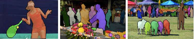
Deep learning algorithms have solved several computer vision tasks with an increasing level of difficulty. In my previous blog posts, I have detailled the well kwown ones: image classification and object detection. The image semantic segmentation challenge consists in classifying each pixel of an image (or just several ones) into an instance, each instance (or category) corresponding to an object or a part of the image (road, sky, …). This task is part of the concept of scene understanding: how a deep learning model can better learn the global context of a visual content ?
The object detection task has exceeded the image classification task in term of complexity. It consists in creating bounding boxes around the objects contained in an image and classify each one of them. Most of the object detection models use anchor boxes and proposals to detect bounding box around objects. Unfortunately, just a few models take into account the entire context of an image but they only classify a small part of the information. Thus, they can’t provide a full comprehension of a scene.
In order to understand a scene, each visual information has to be associated to an entity while considering the spatial information. Several other challenges have emerged to really understand the actions in a image or a video: keypoint detection, action recognition, video captioning, visual question answering and so on. A better comprehension of the environment will help in many fields. For example, an autonomous car needs to delimitate the roadsides with a high precision in order to move by itself. In robotics, production machines should understand how to grab, turn and put together two different pieces requiring to delimitate the exact shape of the object.
In this blog post, architecture of a few previous state-of-the-art models on image semantic segmentation challenges are detailed. Note that researchers test their algorithms using different datasets (PASCAL VOC, PASCAL Context, COCO, Cityscapes) which are different between the years and use different metrics of evaluation. Thus the cited performances cannot be directly compared per se. Moreover, the results depend on the pretrained top network (the backbone), the results published in this post correspond to the best scores published in each paper with respect to their test dataset.
Datasets and Metrics
PASCAL Visual Object Classes (PASCAL VOC)
The PASCAL VOC dataset (2012) is well-known an commonly used for object detection and segmentation. More than 11k images compose the train and validation datasets while 10k images are dedicated to the test dataset.
The segmentation challenge is evaluated using the mean Intersection over Union (mIoU) metric. The Intersection over Union (IoU) is a metric also used in object detection to evaluate the relevance of the predicted locations. The IoU is the ratio between the area of overlap and the area of union between the ground truth and the predicted areas. The mIoU is the average between the IoU of the segmented objects over all the images of the test dataset.


PASCAL-Context
The PASCAL-Context dataset (2014) is an extension of the 2010 PASCAL VOC dataset. It contains around 10k images for training, 10k for validation and 10k for testing. The specificity of this new release is that the entire scene is segmented providing more than 400 categories. Note that the images have been annotated during three months by six in-house annotators.
The official evaluation metric of the PASCAL-Context challenge is the mIoU. Several other metrics are published by researches as the pixel Accuracy (pixAcc). Here, the performances will be compared only with the mIoU.


Common Objects in COntext (COCO)
There are two COCO challenges (in 2017 and 2018) for image semantic segmentation (“object detection” and “stuff segmentation”). The “object detection” task consists in segmenting and categorizing objects into 80 categories. The “stuff segmentation” task uses data with large segmented part of the images (sky, wall, grass), they contain almost the entire visual information. In this blog post, only the results of the “object detection” task will be compared because too few of the quoted research papers have published results on the “stuff segmentation” task.
The COCO dataset for object segmentation is composed of more than 200k images with over 500k object instance segmented. It contains a training dataset, a validation dataset, a test dataset for reseachers (test-dev) and a test dataset for the challenge (test-challenge). The annotations of both test datasets are not available. These datasets contain 80 categories and only the corresponding objects are segmented. This challenge uses the same metrics than the object detection challenge: the Average Precision (AP) and the Average Recall (AR) both using the Intersection over Union (IoU).
Details about IoU and AP metrics are available in my previous blog post. Such as the AP, the Average Recall is computed using multiple IoU with a specific range of overlapping values. For a fixed IoU, the objects with the corresponding test / ground truth overlapping are kept. Then the Recall metric is computed for the detected objects. The final AR metric is the average of the computed Recalls for all the IoU range values. Basically the AP and the AR metrics for segmentation works the same way with object detection excepting that the IoU is computed pixel-wise with a non rectangular shape for semantic segmentation.

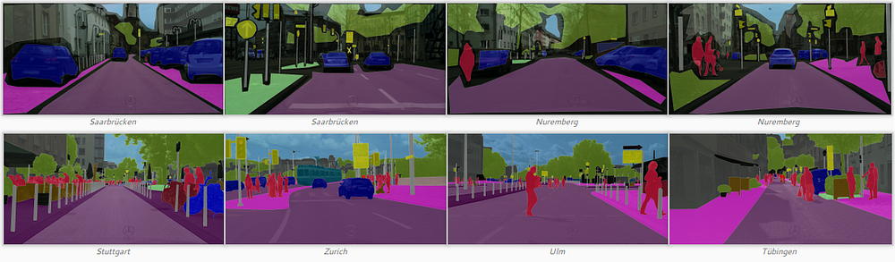
Cityscapes
The Cityscapes dataset has been released in 2016 and consists in complex segmented urban scenes from 50 cities. It is composed of 23.5k images for training and validation (fine and coarse annotations) and 1.5 images for testing (only fine annotation). The images are fully segmented such as the PASCAL-Context dataset with 29 classes (within 8 super categories: flat, human, vehicle, construction, object, nature, sky, void). It is often used to evaluate semantic segmentation models because of its complexity. It is also well known for its similarity with real urban scenes for autonomous driving applications. The performances of semantic segmentation models are computed using the mIoU metric such as the PASCAL datasets.

Fully Convolutional Network (FCN)
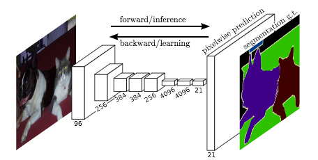
J. Long et al. (2015) have been the firsts to develop an Fully Convolutional Network (FCN) (containing only convolutional layers) trained end-to-end for image segmentation.
The FCN takes an image with an arbitrary size and produces a segmented image with the same size. The authors start by modifying well-known architectures (AlexNet, VGG16, GoogLeNet) to have a non fixed size input while replacing all the fully connected layers by convolutional layers. Since the network produces several feature maps with small sizes and dense representations, an upsampling is necessary to create an output with the same size than the input. Basically, it consists in a convolutional layer with a stride inferior to 1. It is commonly called deconvolution because it creates an output with a larger size than the input. This way, the network is trained using a pixel-wise loss. Moreover they have added skip connections in the network to combine high level feature map representations with more specific and dense ones at the top of the network.
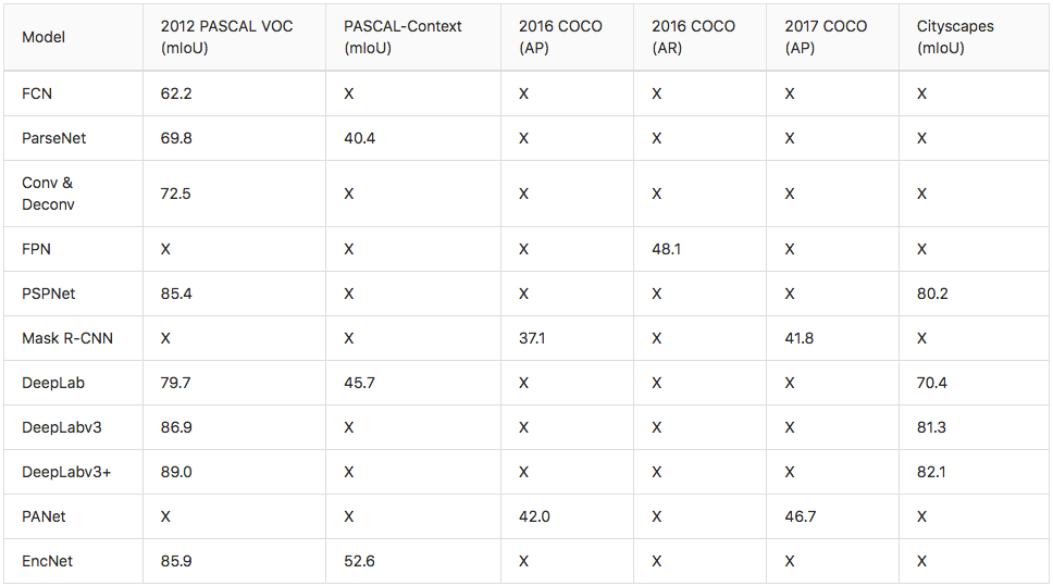
The authors have reached a 62.2% mIoU score on the 2012 PASCAL VOC segmentation challenge using pretrained models on the 2012 ImageNet dataset. For the 2012 PASCAL VOC object detection challenge, the benchmark model called Faster R-CNN has reached 78.8% mIoU. Even if we can’t directly compare the two results (different models, different datasets and different challenges), it seems that the semantic segmentation task is more difficult to solve than the object detection task.

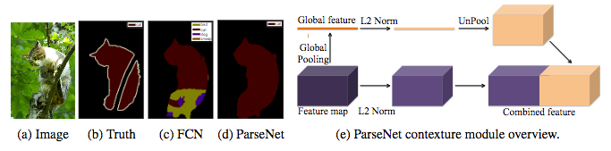
ParseNet
W. Liu et al. (2015) have published a paper explaining improvements of the FCN model of J. Long et al. (2015). According to the authors, the FCN model loses the global context of the image in its deep layers by specializing the generated feature maps. The ParseNet is an end-to-end convolutional network predicting values for all the pixels at the same time and it avoids taking regions as input to keep the global information. The authors use a module taking feature maps as input. The first step uses a model to generate feature maps which are reduced into a single global feature vector with a pooling layer. This context vector is normalised using the L2 Euclidian Norm and it is unpooled (the output is an expanded version of the input) to produce new feature maps with the same sizes than the inital ones. The second step normalises the entire initial feature maps using the L2 Euclidian Norm. The last step concatenates the feature maps generated by the two previous steps. The normalisation is helpful to scale the concatenated feature maps values and it leads to better performances. Basically, the ParseNet is a FCN with this module replacing convolutional layers. It has obtained a 40.4% mIoU score on the PASCAL-Context challenge and a 69.8% mIoU score on the 2012 PASCAL VOC segmentation challenge.

Convolutional and Deconvolutional Networks
H. Noh et al. (2015) have released an end-to-end model composed of two linked parts. The first part is a convolutional network with a VGG16 architecture. It takes as input an instance proposal, for example a bounding box generated by an object detection model. The proposal is processed and transformed by a convolutional network to generate a vector of features. The second part is a deconvolutional network taking the vector of features as input and generating a map of pixel-wise probabilities belonging to each class. The deconvolutional network uses unpooling targeting the maxium activations to keep the location of the information in the maps. The second network also uses deconvolution associating a single input to multiple feature maps. The deconvolution expands feature maps while keeping the information dense.

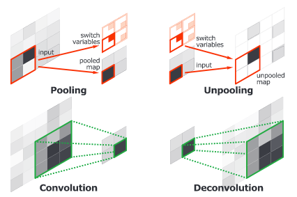
The authors have analysed deconvolution feature maps and they have noted that the low-level ones are specific to the shape while the higher-level ones help to classify the proposal. Finally, when all the proposals of an image are processed by the entire network, the maps are concatenated to obtain the fully segmented image. This network has obtained a 72.5% mIoU on the 2012 PASCAL VOC segmentation challenge.


U-Net
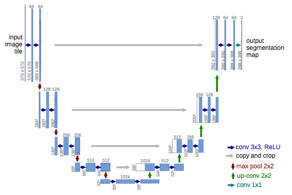
O. Ronneberger et al. (2015) have extended the FCN of J. Long et al. (2015) for biological microscopy images. The authors have created a network called U-net composed in two parts: a contracting part to compute features and a expanding part to spatially localise patterns in the image. The downsampling or contracting part has a FCN-like archicture extracting features with 3x3 convolutions. The upsampling or expanding part uses up-convolution (or deconvolution) reducing the number of feature maps while increasing their height and width. Cropped feature maps from the downsampling part of the network are copied within the upsampling part to avoid loosing pattern information. Finally, a 1x1 convolution processes the feature maps to generate a segmentation map and thus categorise each pixel of the input image. Since then, the U-net architecture has been widely extended in recent works (FPN, PSPNet, DeepLabv3 and so on). Note that it doesn’t use any fully-connected layer. As consequencies, the number of parameters of the model is reduced and it can be trained with a small labelled dataset (using appropriate data augmentation). For example, the authors have used a public dataset with 30 images for training during their experiments.

Feature Pyramid Network (FPN)
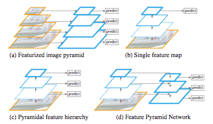
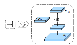
The Feature Pyramid Network (FPN) has been developped by T.-Y. Lin et al (2016) and it is used in object detection or image segmentation frameworks. Its architecture is composed of a bottom-up pathway, a top-down pathway and lateral connections in order to join low-resolution and high-resolution features. The bottom-up pathway takes an image with an arbitrary size as input. It is processed with convolutional layers and downsampled by pooling layers. Note that each bunch of feature maps with the same size is called a stage, the outputs of the last layer of each stage are the features used for the pyramid level. The top-down pathway consists in upsampling the last feature maps with unpooling while enhancing them with feature maps from the same stage of the bottom-up pathway using lateral connections. These connections consist in merging the feature maps of the bottom-up pathway processed with a 1x1 convolution (to reduce their dimensions) with the feature maps of the top-down pathway.

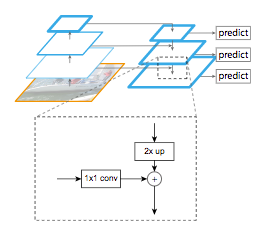
The concatenated feature maps are then processed by a 3x3 convolution to produce the output of the stage. Finally, each stage of the top-down pathway generates a prediction to detect an object. For image segmentation, the authors uses two Multi-Layer Perceptrons (MLP) to generate two masks with different size over the objets. It works similarly to Region Proposal Networks with anchor boxes (R-CNN R. Girshick et al. (2014), Fast R-CNN R. Girshick et al. (2015), Faster R-CNN S. Ren et al. (2016) and so on). This method is efficient because it better propagates low information into the network. The FPN based on DeepMask (P. 0. Pinheiro et al. (2015)) and SharpMask (P. 0. Pinheiro et al. (2016)) frameworks achieved a 48.1% Average Recall (AR) score on the 2016 COCO segmentation challenge.

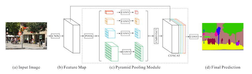
Pyramid Scene Parsing Network (PSPNet)
H. Zhao et al. (2016) have developped the Pyramid Scene Parsing Network (PSPNet) to better learn the global context representation of a scene. Patterns are extracted from the input image using a feature extractor (ResNet K. He et al. (2015)) with a dilated network strategy¹. The feature maps feed a Pyramid Pooling Module to distinguish patterns with different scales. They are pooled with four different scales each one corresponding to a pyramid level and processed by a 1x1 convolutional layer to reduce their dimensions. This way each pyramid level analyses sub-regions of the image with different location. The outputs of the pyramid levels are upsampled and concatenated to the inital feature maps to finally contain the local and the global context information. Then, they are processed by a convolutional layer to generate the pixel-wise predictions. The best PSPNet with a pretrained ResNet (using the COCO dataset) has reached a 85.4% mIoU score on the 2012 PASCAL VOC segmentation challenge.

Mask R-CNN
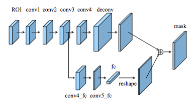
K. He et al. (2017) have released the Mask R-CNN model beating all previous benchmarks on many COCO challenges². I have already provided details about Mask R-CNN for object detection in my previous blog post. As a reminder, the Faster R-CNN (S. Ren et al. (2015)) architecture for object detection uses a Region Proposal Network (RPN) to propose bounding box candidates. The RPN extracts Region of Interest (RoI) and a RoIPool layer computes features from these proposals in order to infer the bounding box cordinates and the class of the object. The Mask R-CNN is a Faster R-CNN with 3 output branches: the first one computes the bounding box coordinates, the second one computes the associated class and the last one computes the binary mask³ to segment the object. The binary mask has a fixed size and it is generated by a FCN for a given RoI. It also uses a RoIAlign layer instead of a RoIPool to avoid misalignments due to the quantization of the RoI coordinates. The particularity of the Mask R-CNN model is its multi-task loss combining the losses of the bounding box coordinates, the predicted class and the segmentation mask. The model tries to solve complementary tasks leading to better performances on each individual task. The best Mask R-CNN uses a ResNeXt (S. Xie et al. (2016)) to extract features and a FPN architecture. It has obtained a 37.1% AP score on the 2016 COCO segmentation challenge and a 41.8% AP score on the 2017 COCO segmentation challenge.


DeepLab, DeepLabv3 and DeepLabv3+
DeepLab
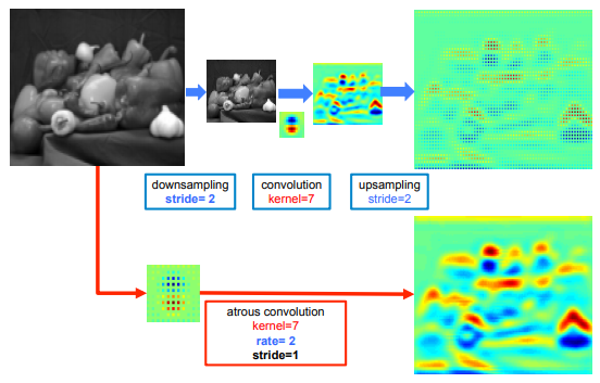
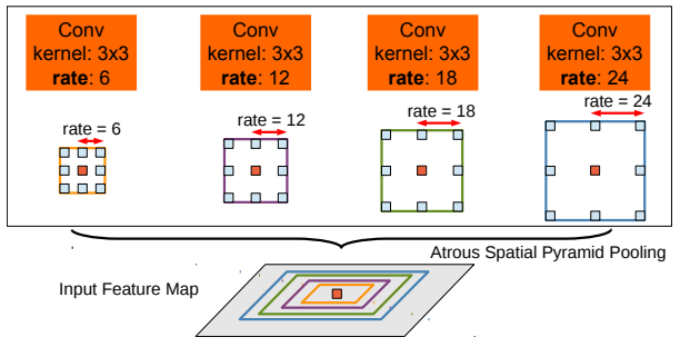
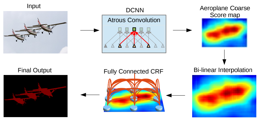
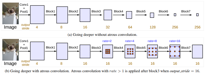
Inspired by the FPN model of T.-Y. Lin et al (2016), L.-C. Chen et al. (2017) have released DeepLab combining atrous convolution, spatial pyramid pooling and fully connected CRFs. The model presented in this paper is also called the DeepLabv2 because it is an adjustment of the initial DeepLab model (details about the inital one will not be provided to avoid redundancy). According to the authors, consecutive max-pooling and striding reduces the resolution of the feature maps in deep neural networks. They have introduced the atrous convolution which is basically the dilated convolution of H. Zhao et al. (2016). It consists of filters targeting sparse pixels with a fixed rate. For example, if the rate is equal to 2, the filter targets one pixel over two in the input; if the rate equal to 1, the atrous convolution is a basic convolution. Atrous convolution permits to capture multiple scale of objects. When it is used without max-poolling, it increases the resolution of the final output without increasing the number of weights.

The Atrous Spatial Pyramid Pooling consists in applying several atrous convolution of the same input with different rate to detect spatial patterns. The features maps are processed in separate branches and concatenated using bilinear interpolation to recovert the original size of the input. The output feeds a fully connected Conditional Random Field (CRF) (Krähenbühl and V. Koltun (2012)) computing edges between the features and long terme dependencies to produce the semantic segmentation.

The best DeepLab using a ResNet-101 as backbone has reached a 79.7% mIoU score on the 2012 PASCAL VOC challenge, a 45.7% mIoU score on the PASCAL-Context challenge and a 70.4% mIoU score on the Cityscapes challenge.

DeepLabv3
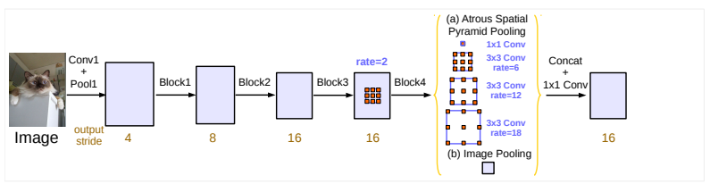
L.-C. Chen et al. (2017) have revisited the DeepLab framework to create DeepLabv3 combining cascaded and parallel modules of atrous convolutions. The authors have modified the ResNet architecture to keep high resolution feature maps in deep blocks using atrous convolutions.

The parallel atrous convolution modules are grouped in the Atrous Spatial Pyramid Pooling (ASPP). A 1x1 convolution and batch normalisation are added in the ASPP. All the outputs are concatenated and processed by another 1x1 convolution to create the final output with logits for each pixel.

The best DeepLabv3 model with a ResNet-101 pretrained on ImageNet and JFT-300M datasets has reached 86.9% mIoU score in the 2012 PASCAL VOC challenge. It also achieved a 81.3% mIoU score on the Cityscapes challenge with a model only trained with the associated training dataset.
DeepLabv3+
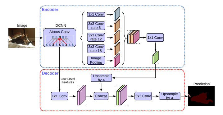
L.-C. Chen et al. (2018) have finally released the Deeplabv3+ framework using an encoder-decoder structure. The authors have introduced the atrous separable convolution composed of a depthwise convolution (spatial convolution for each channel of the input) and pointwise convolution (1x1 convolution with the depthwise convolution as input).

They have used the DeepLabv3 framework as encoder. The most performant model has a modified Xception (F. Chollet (2017)) backbone with more layers, atrous depthwise separable convolutions instead of max pooling and batch normalization. The outputs of the ASPP are processed by a 1x1 convolution and upsampled by a factor of 4. The outputs of the encoder backbone CNN are also processed by another 1x1 convolution and concatenated to the previous ones. The feature maps feed two 3x3 convolutional layers and the outputs are upsampled by a factor of 4 to create the final segmented image.

The best DeepLabv3+ pretrained on the COCO and the JFT datasets has obtained a 89.0% mIoU score on the 2012 PASCAL VOC challenge. The model trained on the Cityscapes dataset has reached a 82.1% mIoU score for the associated challenge.
Path Aggregation Network (PANet)
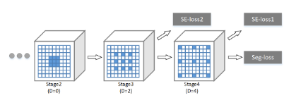
S. Liu et al. (2018) have recently released the Path Aggregation Network (PANet). This network is based on the Mask R-CNN and the FPN frameworks while enhancing information propagation. The feature extractor of the network uses a FPN architecture with a new augmented bottom-up pathway improving the propagation of low-layer features. Each stage of this third pathway takes as input the feature maps of the previous stage and processes them with a 3x3 convolutional layer. The output is added to the same stage feature maps of the top-down pathway using lateral connection and these feature maps feed the next stage.

The feature maps of the augmented bottom-up pathway are pooled with a RoIAlign layer to extract proposals from all level features. An adaptative feature pooling layer processes the features maps of each stage with a fully connected layer and concatenate all the outputs.


The output of the adaptative feature pooling layer feeds three branches similarly to the Mask R-CNN. The two first branches uses a fully connected layer to generate the predictions of the bounding box coordinates and the associated object class. The third branch process the RoI with a FCN to predict a binary pixel-wise mask for the detected object. The authors have added a path processing the output of a convolutional layer of the FCN with a fully connected layer to improve the localisation of the predicted pixels. Finally the output of the parallel path is reshaped and concatenated to the output of the FCN generating the binary mask.

The PANet has achieved 42.0% AP score on the 2016 COCO segmentation challenge using a ResNeXt as feature extractor. They also performed the 2017 COCO segmentation challenge with an 46.7% AP score using a ensemble of seven feature extractors: ResNet (K. He et al. (2015), ResNeXt (S. Xie et al. (2016)) and SENet (J. Hu et al.(2017)).


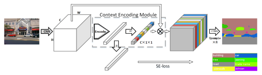
Context Encoding Network (EncNet)
H. Zhang et al. (2018) have created a Context Encoding Network (EncNet) capturing global information in an image to improve scene segmentation. The model starts by using a basic feature extractor (ResNet) and feeds the feature maps into a Context Encoding Module inspired from the Encoding Layer of H. Zhang et al. (2016). Basically, it learns visual centers and smoothing factors to create an embedding taking into account the contextual information while highlighting class-dependant feature maps. On top of the module, scaling factors for the contextual information are learnt with a feature maps attention layer (fully connected layer). In parallel, a Semantic Encoding Loss (SE-Loss) corresponding to a binary cross-entropy loss regularizes the training of the module by detecting presence of object classes (unlike the pixel-wise loss). The outputs of the Context Encoding Module are reshaped and processed by a dilated convolution strategy while minimizing two SE-losses and a final pixel-wise loss. The best EncNet has reached 52.6% mIoU and 81.2% pixAcc scores on the PASCAL-Context challenge. It has also achieved a 85.9% mIoU score on the 2012 PASCAL VOC segmentation challenge.


Conclusion
Image semantic segmentation is a challenge recently takled by end-to-end deep neural networks. One of the main issue between all the architectures is to take into account the global visual context of the input to improve the prediction of the segmentation. The state-of-the-art models use architectures trying to link different part of the image in order to understand the relations between the objects.

The pixel-wise prediction over an entire image allows a better comprehension of the environement with a high precision. Scene understanding is also approached with keypoint detection, action recognition, video captioning or visual question answering. To my opinion, the segmentation task combined with these other issues using multi-task loss should help to outperform the global context understanding of a scene.
Finally, I would like to thanks Long Do Cao for helping me with all my posts, you should check his profile if you’re looking for a great senior data scientist ;).