[深度学习入门]实战二·使用TensorFlow拟合直线

[深度学习入门]实战二·使用TensorFlow拟合直线

• 问题描述

拟合直线 y =（2x -1） + 0.1(-1到1的随机值)
给定x范围（0，3）
可以使用学习框架
建议使用
y = w * x + b 网络模型

• 生成数据

import numpy as np 
import matplotlib.pyplot as plt

def get_data(x,w,b):
    c,r = x.shape
    y = (x * w + b)+ (0.1*(2*np.random.rand(c,r)-1))
    return(y)

xs = np.arange(0,3,0.01).reshape(-1,1)
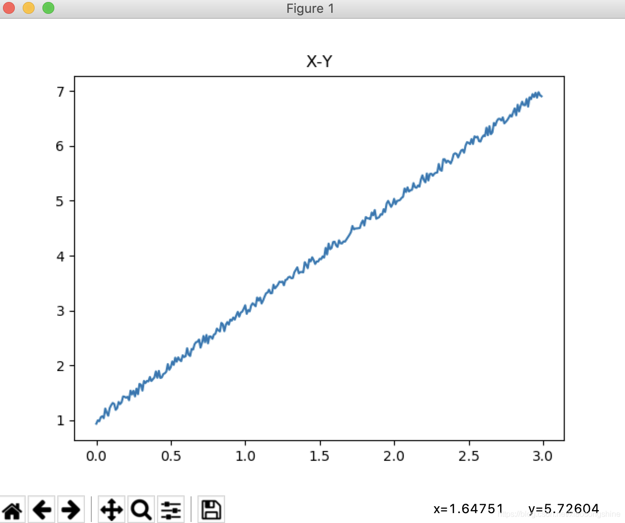
ys = get_data(xs,2,-1)

plt.title("X-Y")
plt.plot(xs,ys)
plt.show()

生成图像：

• 搭建网络结构

x = tf.placeholder(tf.float32,[None,1])
y_ = tf.placeholder(tf.float32,[None,1])

w = tf.get_variable("w1",initializer=tf.random_normal([1,1]))
b = tf.get_variable("b1",initializer=tf.zeros([1,1]))
y = w*x + b

• 定义学习函数

loss = tf.reduce_mean(tf.square(y-y_))
opt = tf.train.GradientDescentOptimizer(0.02).minimize(loss)

• 训练网络参数

with tf.Session() as sess:
    srun = sess.run
    init = tf.global_variables_initializer()
    srun(init)
    print("w0 b0",srun([w,b]))
    for e in range(500):
        loss_val,_ = srun([loss,opt],{x:xs,y_:ys})
        if(e%50 ==0):
            print("%d steps loss is %f",e,loss_val)
    print("w b",srun([w,b]))
    w_pre,b_pre =srun(w)[0,0],srun(b)[0,0]
    print(w_pre,b_pre)

• 显示预测结果

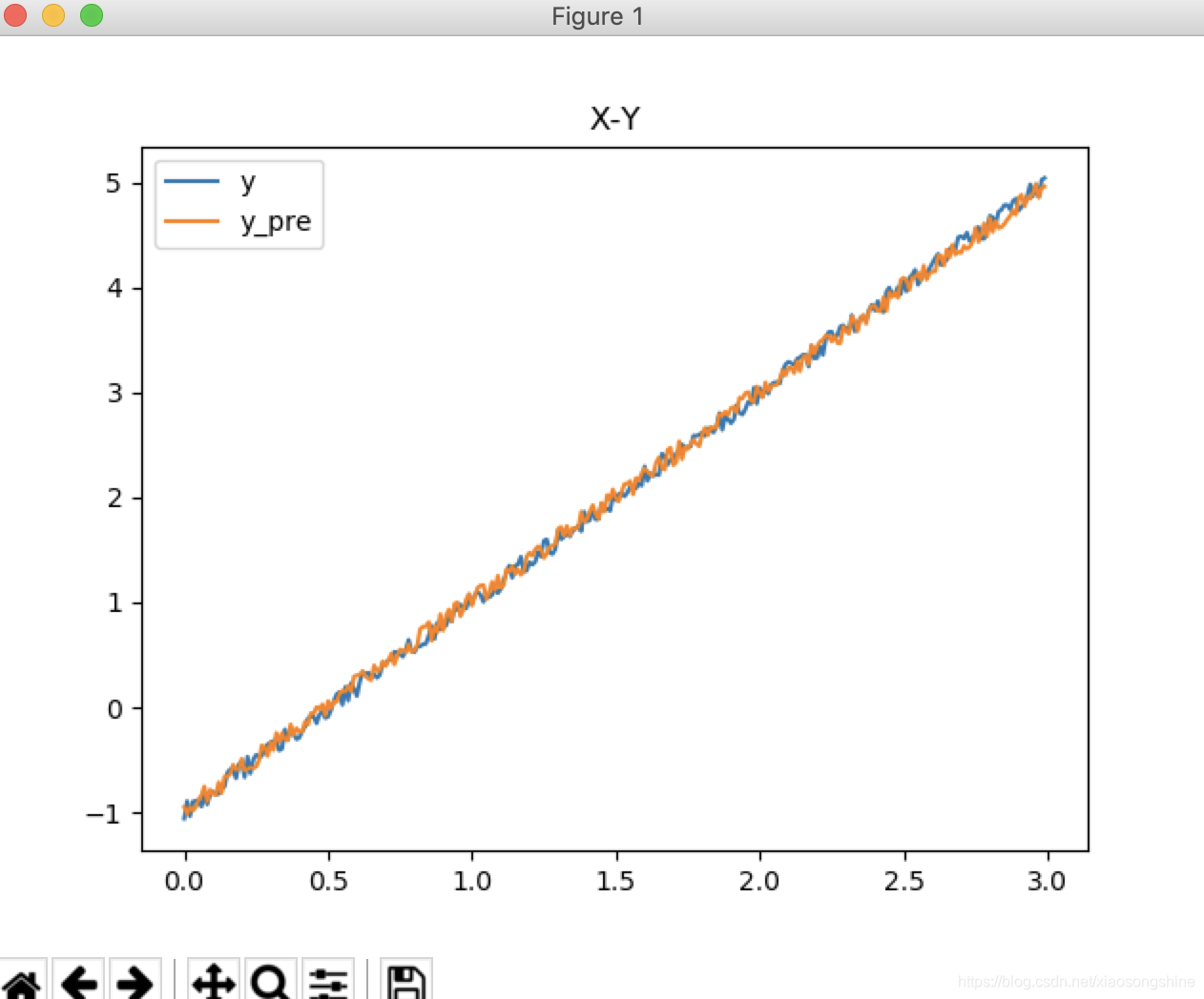
ys_pre = get_data(xs,w_pre,b_pre)
plt.title("X-Y")
plt.plot(xs,ys)
plt.plot(xs,ys_pre)
plt.legend(["y","y_pre"])
plt.show()

• 运行结果
  log：

w0 b0 [array([[-0.4106835]], dtype=float32), array([[0.]], dtype=float32)]
%d steps loss is %f 0 11.149577
%d steps loss is %f 50 0.37165892
%d steps loss is %f 100 0.16953693
%d steps loss is %f 150 0.07829344
%d steps loss is %f 200 0.03710342
%d steps loss is %f 250 0.018508982
%d steps loss is %f 300 0.010114888
%d steps loss is %f 350 0.0063255588
%d steps loss is %f 400 0.0046149325
%d steps loss is %f 450 0.0038427087
w b [array([[1.9863906]], dtype=float32), array([[-0.9746746]], dtype=float32)]
1.9863906 -0.9746746

运行结果图

• 完整代码

import numpy as np 
import matplotlib.pyplot as plt
import tensorflow as tf



def get_data(x,w,b):
    c,r = x.shape
    y = (x * w + b)+ (0.1*(2*np.random.rand(c,r)-1))
    return(y)

xs = np.arange(0,3,0.01).reshape(-1,1)
ys = get_data(xs,2,-1)

print(ys.shape)
"""plt.title("X-Y")
plt.plot(xs,ys)
plt.show()"""

x = tf.placeholder(tf.float32,[None,1])
y_ = tf.placeholder(tf.float32,[None,1])

w = tf.get_variable("w1",initializer=tf.random_normal([1,1]))
b = tf.get_variable("b1",initializer=tf.zeros([1,1]))
y = w*x + b

loss = tf.reduce_mean(tf.square(y-y_))
opt = tf.train.GradientDescentOptimizer(0.02).minimize(loss)

with tf.Session() as sess:
    srun = sess.run
    init = tf.global_variables_initializer()
    srun(init)
    print("w0 b0",srun([w,b]))
    for e in range(500):
        loss_val,_ = srun([loss,opt],{x:xs,y_:ys})
        if(e%50 ==0):
            print("%d steps loss is %f",e,loss_val)
    print("w b",srun([w,b]))
    w_pre,b_pre =srun(w)[0,0],srun(b)[0,0]
    print(w_pre,b_pre)

ys_pre = get_data(xs,w_pre,b_pre)
plt.title("X-Y")
plt.plot(xs,ys)
plt.plot(xs,ys_pre)
plt.legend(["y","y_pre"])
plt.show()