[深度学习入门]实战三·使用TensorFlow拟合曲线

问题描述
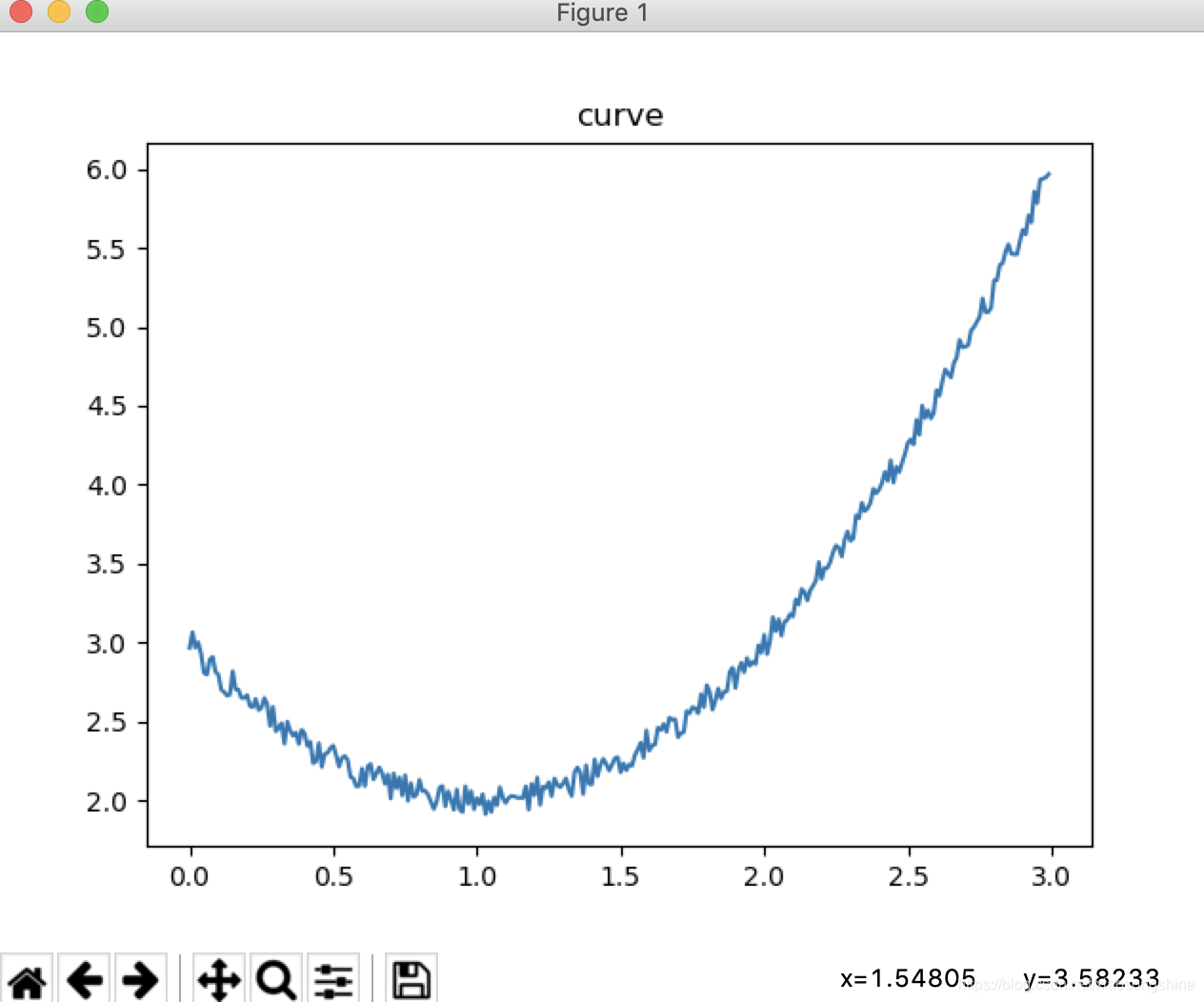
拟合y= x*x -2x +3 + 0.1(-1到1的随机值) 曲线
给定x范围（0，3）
问题分析
在上篇博客中，我们使用最简单的y=wx+b的模型成功拟合了一条直线，现在我们在进一步进行曲线的拟合。简单的y=wx+b模型已经无法满足我们的需求，需要利用更多的神经元来解决问题了。
生成数据

import numpy as np 
import matplotlib.pyplot as plt
import tensorflow as tf

def get_data(x,w,b,d):
    c,r = x.shape
    y = (w * x * x + b*x + d)+ (0.1*(2*np.random.rand(c,r)-1))
    return(y)
xs = np.arange(0,3,0.01).reshape(-1,1)
ys = get_data(xs,1,-2,3)
plt.title("curve")
plt.plot(xs,ys)
plt.show()

生成的数据图像为：
在这里插入图片描述

搭建网络结构

x = tf.placeholder(tf.float32,[None,1])
y_ = tf.placeholder(tf.float32,[None,1])

w1 = tf.get_variable("w1",initializer=tf.random_normal([1,16]))
w2 = tf.get_variable("w2",initializer=tf.random_normal([16,1]))
b1 = tf.get_variable("b1",initializer=tf.zeros([1,16]))
b2 = tf.get_variable("b2",initializer=tf.zeros([1,1]))
l1 = tf.matmul(x,w1)+b1
l1 = tf.nn.elu(l1)
y = tf.matmul(l1,w2)+b2

定义学习函数

loss = tf.reduce_mean(tf.square(y-y_))
opt = tf.train.GradientDescentOptimizer(0.02).minimize(loss)

训练网络参数

with tf.Session() as sess:
    srun = sess.run
    init = tf.global_variables_initializer()
    srun(init)
    
    for e in range(4001):
        loss_val,_ = srun([loss,opt],{x:xs,y_:ys})
        if(e%200 ==0):
            print("%d steps loss is %f"%(e,loss_val))

    ys_pre = srun(y,{x:xs})

显示预测结果

plt.title("curve")
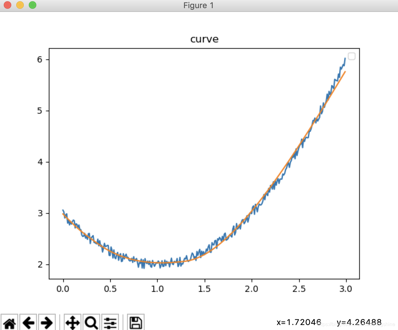
plt.plot(xs,ys)
plt.plot(xs,ys_pre)
plt.legend("ys","ys_pre")
plt.show()

运行结果
log：

0 steps loss is 49.556065
200 steps loss is 0.352589
400 steps loss is 0.108551
600 steps loss is 0.042510
800 steps loss is 0.030316
1000 steps loss is 0.024551
1200 steps loss is 0.020459
1400 steps loss is 0.017488
1600 steps loss is 0.015306
1800 steps loss is 0.013710
2000 steps loss is 0.012510
2200 steps loss is 0.011569
2400 steps loss is 0.010802
2600 steps loss is 0.010148
2800 steps loss is 0.009566
3000 steps loss is 0.009039
3200 steps loss is 0.008552
3400 steps loss is 0.008097
3600 steps loss is 0.007674
3800 steps loss is 0.007285
4000 steps loss is 0.006934

运行结果图
在这里插入图片描述

完整代码

import os
os.environ["KMP_DUPLICATE_LIB_OK"]="TRUE"
import numpy as np 
import matplotlib.pyplot as plt
import tensorflow as tf

def get_data(x,w,b,d):
    c,r = x.shape
    y = (w * x * x + b*x + d)+ (0.1*(2*np.random.rand(c,r)-1))
    return(y)

xs = np.arange(0,3,0.01).reshape(-1,1)
ys = get_data(xs,1,-2,3)
"""plt.title("curve")
plt.plot(xs,ys)
plt.show()"""

x = tf.placeholder(tf.float32,[None,1])
y_ = tf.placeholder(tf.float32,[None,1])

w1 = tf.get_variable("w1",initializer=tf.random_normal([1,16]))
w2 = tf.get_variable("w2",initializer=tf.random_normal([16,1]))
b1 = tf.get_variable("b1",initializer=tf.zeros([1,16]))
b2 = tf.get_variable("b2",initializer=tf.zeros([1,1]))
l1 = tf.matmul(x,w1)+b1
l1 = tf.nn.elu(l1)
y = tf.matmul(l1,w2)+b2

loss = tf.reduce_mean(tf.square(y-y_))
opt = tf.train.GradientDescentOptimizer(0.02).minimize(loss)

with tf.Session() as sess:
    srun = sess.run
    init = tf.global_variables_initializer()
    srun(init)
    
    for e in range(4001):
        loss_val,_ = srun([loss,opt],{x:xs,y_:ys})
        if(e%200 ==0):
            print("%d steps loss is %f"%(e,loss_val))

    ys_pre = srun(y,{x:xs})

plt.title("curve")
plt.plot(xs,ys)
plt.plot(xs,ys_pre)
plt.legend("ys","ys_pre")
plt.show()

[深度学习入门]实战三·使用TensorFlow拟合曲线

[深度学习入门]实战三·使用TensorFlow拟合曲线

猜你喜欢