实验指导书 下载密码:hso0
本篇博客主要讲解,吴恩达机器学习第二周的编程作业,作业内容主要是实现单元/多元线性回归算法。实验的原始版本是用Matlab实现的,本篇博客主要用Python来实现。
目录
1.实验包含的文件

| 文件名称 | 含义 |
| ex1.py | 单元线性回归的主程序 |
| ex1_multi.py | 多元线性回归主程序 |
| ex1data1.txt | 单变量线性回归数据集 |
| ex1data2.txt | 多变量线性回归数据集 |
| plotData.py | 可视化数据集程序 |
| computeCost.py | 计算线性回归的代价函数程序 |
| gradientDescent.py | 梯度下降法程序 |
| featureNormalize.py | 特征缩放程序 |
| normalEqn.py | 正规方程求解线性回归程序 |
实验任务完成红色部分程序的关键代码。
2.单元线性回归
- 任务:预测快餐车的收益,输入变量只有一个特征是城市的人口,输出变量是快餐车在该城市的收益。
- 打开单元线性回归主程序ex1.py
'''第1部分 可视化训练集'''
print('Plotting Data...')
data = np.loadtxt('ex1data1.txt', delimiter=',', usecols=(0, 1))#加载txt格式的数据集 每一行以","分隔
X = data[:, 0]   #输入变量 第一列
y = data[:, 1]   #输出变量 第二列
m = y.size     #样本数

plt.ion()
plt.figure(0)
plot_data(X, y) #可视化数据集- 编写可视化程序plotData.py
def plot_data(x, y):

    plt.scatter(x,y,marker='o',s=50,cmap='Blues',alpha=0.3)  #绘制散点图
    plt.xlabel('population')  #设置x轴标题
    plt.ylabel('profits')   #设置y轴标题

plt.show()- 可视化效果

- 使用梯度下降法求解单元线性回归
'''第2部分 梯度下降法'''
print('Running Gradient Descent...')
X = np.c_[np.ones(m), X] # 输入特征矩阵 前面增加一列1 方便矩阵运算
theta = np.zeros(2) # 初始化两个参数为0
iterations = 1500 #设置梯度下降迭代次数
alpha = 0.01 #设置学习率
# 计算最开始的代价函数值 并与期望值比较 验证程序正确性
print('Initial cost : ' + str(compute_cost(X, y, theta)) + ' (This value should be about 32.07)')
#使用梯度下降法求解线性回归 返回最优参数 以及每一步迭代后的代价函数值
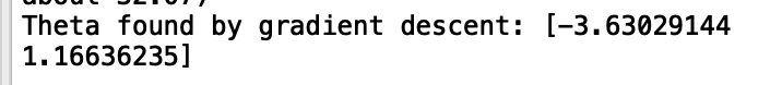
theta, J_history = gradient_descent(X, y, theta, alpha, iterations)
print('Theta found by gradient descent: ' + str(theta.reshape(2)))
# 在数据集上绘制出拟合的直线
plt.figure(0)
line1, = plt.plot(X[:, 1], np.dot(X, theta), label='Linear Regression')
plt.legend(handles=[line1])
input('Program paused. Press ENTER to continue')
# 用训练好的参数 预测人口为3.5*1000时 收益为多少 并与期望值比较 验证程序正确性
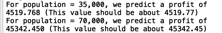
predict1 = np.dot(np.array([1, 3.5]), theta)
print('For population = 35,000, we predict a profit of {:0.3f} (This value should be about 4519.77)'.format(predict1*10000))
# 用训练好的参数 预测人口为7*1000时 收益为多少 并与期望值比较 验证程序正确性
predict2 = np.dot(np.array([1, 7]), theta)
print('For population = 70,000, we predict a profit of {:0.3f} (This value should be about 45342.45)'.format(predict2*10000))
- 编写计算线性回归代价函数的程序computeCost.py

def h(X,theta): #线性回归假设函数
return X.dot(theta)
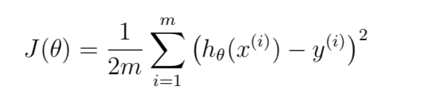
def compute_cost(X, y, theta):
m = y.size #样本数
cost = 0 #代价函数值
myh=h(X,theta) #得到假设函数值 (m,)
cost=(myh-y).dot(myh-y)/(2*m) #计算代价函数值
return cost
与期望值进行比较,说明我们编写的计算代价函数的代码是正确的。
- 编写梯度下降法程序gradientDescent.py
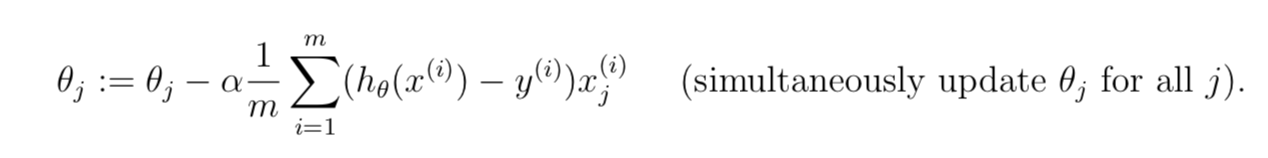
def gradient_descent(X, y, theta, alpha, num_iters):

    m = y.size #样本数
    J_history = np.zeros(num_iters)  #每一次迭代都有一个代价函数值

    for i in range(0, num_iters):   #num_iters次迭代优化
        theta=theta-(alpha/m)*(h(X,theta)-y).dot(X)
        J_history[i] = compute_cost(X, y, theta) #用每一次迭代产生的参数 来计算代价函数值

    return theta, J_history
梯度下降法求解的最优参数值:
利用训练好的参数进行预测,与期望值进行比较,验证我们的程序是正确的:
在数据集上可视化拟合的直线:

- 根据不同的参数取值,可视化代价函数
'''第3部分 可视化代价函数'''
print('Visualizing J(theta0, theta1) ...')

theta0_vals = np.linspace(-10, 10, 100)  #参数1的取值
theta1_vals = np.linspace(-1, 4, 100)    #参数2的取值

xs, ys = np.meshgrid(theta0_vals, theta1_vals)   #生成网格
J_vals = np.zeros(xs.shape)


for i in range(0, theta0_vals.size):
    for j in range(0, theta1_vals.size):
        t = np.array([theta0_vals[i], theta1_vals[j]])
        J_vals[i][j] = compute_cost(X, y, t)    #计算每个网格点的代价函数值

J_vals = np.transpose(J_vals)

fig1 = plt.figure(1)      #绘制3d图形
ax = fig1.gca(projection='3d')
ax.plot_surface(xs, ys, J_vals)
plt.xlabel(r'$\theta_0$')
plt.ylabel(r'$\theta_1$')

#绘制等高线图 相当于3d图形的投影
plt.figure(2)
lvls = np.logspace(-2, 3, 20)
plt.contour(xs, ys, J_vals, levels=lvls, norm=LogNorm())
plt.plot(theta[0], theta[1], c='r', marker="x")
可视化效果:

3.单元线性回归完整项目代码
下载链接 下载密码:d8dd
4.多元线性回归
- 任务:预测房价,输入变量有两个特征,一是房子的面积,二是房子卧室的数量;输出变量是房子的价格。
- 打开多元线性回归主程序ex1_multi.py
'''第1部分 特征缩放'''
print('Loading Data...')
data = np.loadtxt('ex1data2.txt', delimiter=',', dtype=np.int64)#加载txt格式数据集 每一行以','分隔
X = data[:, 0:2]   #得到输入变量矩阵  每个输入变量有两个输入特征
y = data[:, 2]   #输出变量
m = y.size  #样本数

# 打印前10个训练样本
print('First 10 examples from the dataset: ')
for i in range(0, 10):
    print('x = {}, y = {}'.format(X[i], y[i]))

input('Program paused. Press ENTER to continue')

# 特征缩放  不同特征的取值范围差异很大  通过特征缩放 使其在一个相近的范围内
print('Normalizing Features ...')

X, mu, sigma = feature_normalize(X)
X = np.c_[np.ones(m), X] # 得到缩放后的特征矩阵 前面加一列1 方便矩阵运算- 编写特征缩放程序featureNormalize.py
def feature_normalize(X):

    n = X.shape[1]  # shape[1]返回特征矩阵列数 即特征数
    X_norm = X     #初始化特征缩放后的特征矩阵
    mu = np.zeros(n)  #初始化每一列特征的均值
    sigma = np.zeros(n)  #初始化每一列特征的标准差

    mu=np.mean(X,axis=0) #对每一列求均值
    sigma=np.std(axis=0) #对每一列求标准差
    X_norm=(X_norm-mu)/sig #广播 每一列减去该列的均值/该列的标准差

    return X_norm, mu, sigma
- 使用梯度下降法求解最优参数并进行预测,绘制代价函数随迭代次数的变化曲线
'''第2部分 梯度下降法'''


print('Running gradient descent ...')


alpha = 0.03  #学习率
num_iters = 400 #迭代次数


theta = np.zeros(3)#初始化参数
theta, J_history = gradient_descent_multi(X, y, theta, alpha, num_iters) #梯度下降求解参数

# 绘制代价函数值随迭代次数的变化曲线
plt.figure()
plt.plot(np.arange(J_history.size), J_history)
plt.xlabel('Number of iterations')
plt.ylabel('Cost J')

# 打印求解的最优的参数
print('Theta computed from gradient descent : \n{}'.format(theta))

# 预测面积是1650 卧室数是3 的房子的价格

x1=np.array([1650,3])

x1=(x1-mu)/sigma  #对预测样例进行特征缩放
x1=np.r_[1,x1]  #前面增加一个1
price = h(x1,theta)  #带入假设函数 求解预测值


# ==========================================================

print('Predicted price of a 1650 sq-ft, 3 br house (using gradient descent) : {:0.3f}'.format(price))- 编写计算线性回归代价函数的程序computeCost.py
def h(X,theta):  #线性回归假设函数
    return X.dot(theta)

def compute_cost(X, y, theta):

    m = y.size #样本数
    cost = 0   #代价函数值
    myh=h(X,theta)  #得到假设函数值  (m,)

    cost=(myh-y).dot(myh-y)/(2*m)  #计算代价函数值

return cost- 编写梯度下降法程序gradientDescent.py
def gradient_descent_multi(X, y, theta, alpha, num_iters):

    m = y.size #样本数
    J_history = np.zeros(num_iters)  #每一次迭代都有一个代价函数值

    for i in range(0, num_iters):   #num_iters次迭代优化
        theta=theta-(alpha/m)*(h(X,theta)-y).dot(X)
        J_history[i] = compute_cost(X, y, theta) #用每一次迭代产生的参数 来计算代价函数值

    return theta, J_history
- 梯度下降法求解的最优参数,样例的预测价格以及代价函数随迭代次数的变化曲线

- 利用正规方程法求解多元线性回归,并预测样例的房价
'''第3部分 正规方程法求解多元线性回归'''
#正规方程法不用进行特征缩放

print('Solving with normal equations ...')


# Load data
data = np.loadtxt('ex1data2.txt', delimiter=',', dtype=np.int64)
X = data[:, 0:2]
y = data[:, 2]
m = y.size

# 增加一列特征1
X = np.c_[np.ones(m), X]

theta = normal_eqn(X, y) #正规方程法

# 打印求解的最优参数
print('Theta computed from the normal equations : \n{}'.format(theta))

# 预测面积是1650 卧室数是3 的房子的价格

x2=np.array([1,1650,3])
price = h(x2,theta) #带入假设函数 求解预测值


# ==========================================================

print('Predicted price of a 1650 sq-ft, 3 br house (using normal equations) : {:0.3f}'.format(price))- 编写正规方程法程序 normalEqn.py

def normal_eqn(X, y):
    theta = np.zeros((X.shape[1], 1))

    theta=inv(X.T.dot(X)).dot(X.T).dot(y)


    return theta
- 正规方程法求解的最优参数,和预测样例的房价

可以看到两种方法预测的房价差不多。
5.多元线性回归完整项目代码
下载链接 下载密码:cz04