Python学习--Machine-Learning 吴恩达机器学习编程作业 (第四周)

Machine-Learning 编程作业

Programming Exercise 4：Neural Network Learning

神经网络的实现

这部分完成的是利用练习三中的数据，随机初始化参数，从头开始实现手写数字的识别，最终利用我们训练好的模型进行预测，并给出准确率。
步骤分为：
1. 导入数据并可视化
2. 标签向量化
3. 定义前向传播函数
4. 定义代价函数+反向传播函数
5. 初始化参数
6. 用高级函数最小化目标函数
7. 隐藏层可视化

作业文件打包如下： 链接：https://pan.baidu.com/s/1S6-q29v_zYWUXugWAZk-zg 提取码：h20r

导入数据并可视化

首先，这与上一次练习中使用的数据集相同。在ex3data1.mat中有5000个训练示例，其中每个训练示例是20×20像素的数字灰度图像。像素用浮点数表示，表示该位置的灰度强度。所有20×20像素的训练图像都被“展开”成400维矢量，形成了5000×400的矩阵X，其中每一行都是一个手写数字图像的训练示例。训练集的第二部分是包含训练集标签的5000维向量y。数字“0”被标记为“10”，而数字“1”到“9”则被标记为“1”到“9”。

#!/usr/bin/env python
# -*- coding:utf-8 -*-

import numpy as np
import matplotlib.pyplot as plt
from scipy.io import loadmat
import matplotlib
import scipy.optimize as opt
from sklearn.metrics import classification_report

data = loadmat('ex4data1.mat')
X = data['X']
y = data['y']
print(X.shape, y.shape)

#可视化数据部分
def display(x):
    (m, n) = x.shape   #100*400
    width = np.round(np.sqrt(n)).astype(int)
    height = (n / width).astype(int)

    gap = 1  #展示图像间的距离
    display_array = -np.ones((gap + 10 * (width + gap), gap + 10 * (height + gap)))
    # 将样本填入到display矩阵中
    curr_ex = 0
    for j in range(10):
        for i in range(10):
            if curr_ex > m:
                break
            # Get the max value of the patch
            max_val = np.max(np.abs(x[curr_ex]))
            display_array[gap + j * (height + gap) + np.arange(height),
                          gap + i * (width + gap) + np.arange(width)[:, np.newaxis]] = \
                x[curr_ex].reshape((height, width)) / max_val
            curr_ex += 1
        if curr_ex > m:
            break
    plt.figure()
    plt.imshow(display_array, cmap='gray', extent=[-1, 1, -1, 1])
    plt.show()

# 随机抽取100个训练样本 进行可视化
m = y.size
rand_indices = np.random.permutation(range(m))  # 获取0-4999 5000个无序随机索引
selected = X[rand_indices[0:100], :]  # 获取前100个随机索引对应的整条数据的输入特征
print(selected.shape)
display(selected)

运行结如下图：

标签向量化

首先我们要将标签值（1，2，3，4，…，10）转化成非线性相关的向量，向量对应位置（y[i-1]）上的值等于1，例如y[0]=4转化为y[0]=[0,0,0,1,0,0,0,0,0,0]。因为网络的输出层有10个输出单元，输出结果是也是对应位为1，其余位为0。下面分两种方法实现，一种自行实现，一种借助函数实现：

# #方法1：
# def expend_y(y):
#     temp = []
#     for i in y:
#         y_array = np.zeros(10)
#         y_array[i - 1] = 1
#         temp.append(y_array)
#     return np.array(temp)
# y_onehot = expend_y(y)
# print(y_onehot.shape)


#方法2：
from sklearn.preprocessing import OneHotEncoder
encoder = OneHotEncoder(sparse=False)
y_onehot = encoder.fit_transform(y)
print(y_onehot.shape)

定义前向传播函数

前向传播示例如图：

#定义前向传播函数
def sigmoid(z):
    return 1 / (1 + np.exp(-z))

#定义前向传播函数
def forward_propagate(X, theta1, theta2):
    m = X.shape[0]

    a1 = np.insert(X, 0, values=np.ones(m), axis=1)
    z2 = a1 * theta1.T
    a2 = np.insert(sigmoid(z2), 0, values=np.ones(m), axis=1)
    z3 = a2 * theta2.T
    h = sigmoid(z3)

    return a1, z2, a2, z3, h

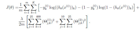
定义代价函数+反向传播函数

带正则化的目标函数如下：

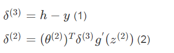
而反向传播函数从后往前计算每层的误差。过程为(第一层为输入层，没有误差)：

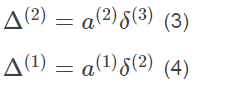
然后计算每层参数矩阵的梯度：

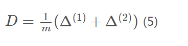
最后总体梯度为：

这里我们直接采用高级优化算法进行优化，所以不写梯度下降函数了。

#计算sigmoid函数的梯度
def sigmoid_gradient(z):
    return np.multiply(sigmoid(z), (1 - sigmoid(z)))

#定义前向传播与后向传播
def backprop(params, input_size, hidden_size, num_labels, X, y, l):
    m = X.shape[0]
    X = np.matrix(X)
    y = np.matrix(y)

    # 将参数数组重新塑造为每个层的参数矩阵
    theta1 = np.matrix(np.reshape(params[:hidden_size * (input_size + 1)], (hidden_size, (input_size + 1))))
    theta2 = np.matrix(np.reshape(params[hidden_size * (input_size + 1):], (num_labels, (hidden_size + 1))))

    # 运行前向传递
    a1, z2, a2, z3, h = forward_propagate(X, theta1, theta2)

    # 赋初值
    J = 0
    delta1 = np.zeros(theta1.shape)  # (25, 401)
    delta2 = np.zeros(theta2.shape)  # (10, 26)

    # 计算代价
    for i in range(m):
        first_term = np.multiply(-y[i, :], np.log(h[i, :]))
        second_term = np.multiply((1 - y[i, :]), np.log(1 - h[i, :]))
        J += np.sum(first_term - second_term)

    J = J / m

    # 添加代价函数正则化项
    J += (float(l) / (2 * m)) * (np.sum(np.power(theta1[:, 1:], 2)) + np.sum(np.power(theta2[:, 1:], 2)))

    # 执行反向传播
    for t in range(m):
        a1t = a1[t, :]  # (1, 401)
        z2t = z2[t, :]  # (1, 25)
        a2t = a2[t, :]  # (1, 26)
        ht = h[t, :]  # (1, 10)
        yt = y[t, :]  # (1, 10)

        d3t = ht - yt  # (1, 10)

        z2t = np.insert(z2t, 0, values=np.ones(1))  # (1, 26)
        d2t = np.multiply((theta2.T * d3t.T).T, sigmoid_gradient(z2t))  # (1, 26)

        delta1 = delta1 + (d2t[:, 1:]).T * a1t
        delta2 = delta2 + d3t.T * a2t

    delta1 = delta1 / m
    delta2 = delta2 / m

    # 添加梯度正则化项
    delta1[:, 1:] = delta1[:, 1:] + (theta1[:, 1:] * l) / m
    delta2[:, 1:] = delta2[:, 1:] + (theta2[:, 1:] * l) / m

    # 将剃度矩阵分解为数组
    grad = np.concatenate((np.ravel(delta1), np.ravel(delta2)))

    return J, grad

J, grad = backprop(params, input_size, hidden_size, num_labels, X, y_onehot, l)
print(J, grad.shape)

初始化参数

# 初始化设置
input_size = 400
hidden_size = 25
num_labels = 10
l = 1

# 随机初始化完整网络参数大小的参数数组
params = (np.random.random(size=hidden_size * (input_size + 1) + num_labels * (hidden_size + 1)) - 0.5) * 0.25

m = X.shape[0]
X = np.matrix(X)
y = np.matrix(y)

# 将参数数组解开为每个层的参数矩阵
theta1 = np.matrix(np.reshape(params[:hidden_size * (input_size + 1)], (hidden_size, (input_size + 1))))
theta2 = np.matrix(np.reshape(params[hidden_size * (input_size + 1):], (num_labels, (hidden_size + 1))))

print(theta1.shape, theta2.shape)
a1, z2, a2, z3, h = forward_propagate(X, theta1, theta2)
print(a1.shape, z2.shape, a2.shape, z3.shape, h.shape)
# print(cost(params, input_size, hidden_size, num_labels, X, y_onehot, l))

输出：

用高级函数最小化目标函数

J, grad = backprop(params, input_size, hidden_size, num_labels, X, y_onehot, l)
print(J, grad.shape)

from scipy.optimize import minimize
#最小化目标函数
fmin = minimize(fun=backprop, x0=params, args=(input_size, hidden_size, num_labels, X, y_onehot, l),
                method='TNC', jac=True, options={'maxiter' : 250})
print(fmin)

X = np.matrix(X)
theta1 = np.matrix(np.reshape(fmin.x[:hidden_size * (input_size + 1)], (hidden_size, (input_size + 1))))
theta2 = np.matrix(np.reshape(fmin.x[hidden_size * (input_size + 1):], (num_labels, (hidden_size + 1))))

a1, z2, a2, z3, h = forward_propagate(X, theta1, theta2)
y_pred = np.array(np.argmax(h, axis=1) + 1)
y_pred

correct = [1 if a == b else 0 for (a, b) in zip(y_pred, y)]
accuracy = (sum(map(int, correct)) / float(len(correct)))
print ('accuracy = {0}%'.format(accuracy * 100))

这里运行结果如下：

隐藏层可视化

最后，进行隐藏层可视化，注意隐藏层有25个隐藏单元(偏置项不算在内)，所以我们要对输出的theta1参数去掉第一列，转换成25×400维矩阵，其中25行代表25个隐藏单元，每一列表示对应某个隐藏单元上的20×20的输出图像。我们将其排列成5×5大小的画板，可视化隐藏层的数据。

#将向量化的参数重组为矩阵
def deserialize(seq):
#     """into ndarray of (25, 401), (10, 26)"""
    return seq[:25 * 401].reshape(25, 401), seq[25 * 401:].reshape(10, 26)

#显示隐藏层
def plot_hidden_layer(theta):
    'theta:  (10285, )'
    final_theta1,final_theta2= deserialize(theta)
    hidden_layer = final_theta1[:, 1:] #去掉偏置项
    fig, ax_array = plt.subplots(nrows=5, ncols=5, sharey=True,
                                 sharex=True, figsize=(5, 5))

    for i in range(5):
        for j in range(5):
            ax_array[i, j].matshow(hidden_layer[5 * i + j].reshape((20, 20)),
                                   cmap=matplotlib.cm.binary)
            plt.xticks(np.array([]))
            plt.yticks(np.array([]))

plot_hidden_layer(fmin.x)
plt.show()

最终隐藏层可视化结果如下：

大功告成！