机器学习笔记——梯度下降（Gradient Descent）

梯度下降算法（Gradient Descent）

在所有的机器学习算法中，并不是每一个算法都能像之前的线性回归算法一样直接通过数学推导就可以得到一个具体的计算公式，而再更多的时候我们是通过基于搜索的方式来求得最优解的，这也是梯度下降法所存在的意义。

• 不是一个机器学习算法
• 是一种基于搜索的最优化方法
• 作用：最小化一个损失函数
• 梯度上升法：最大化一个效用函数

1 梯度下降法

1.1 什么梯度下降法？

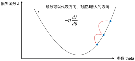
图中任意一点的斜率我们可以用 $\frac{dJ}{d\theta}$来表示，而斜率的正负更可以表示增大或减小的放下，若斜率为正则沿 $x$ 正方向增大，若斜率为负则沿 $x$ 正方向减小，当我们设置一个步长 $\eta$ ，以及一个起始点 $(J,\theta)$ ，每次向 $J$ 减小的方向移动一个步长，则有：
$J(\theta-\eta) \approx J(\theta) -\eta\frac{dJ}{d\theta}$
这样通过搜索的方法就可以找到一个最小的 $J$ ，而对于某些函数来说并不是都存在一个唯一的极值点，例如下图中的情况：

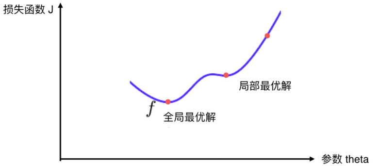
函数 $f$ 存在一个局部最优解和一个全局最优解，按照梯度下降算法，如果我们的起始点选在了最右边的红点处的话那么这样寻找到得只是一个局部最优解。为了解决这个问题，我们通常的做法是多次运行，随机化初始点。因此我们可以知道梯度下降算法中的初始点也是一个超参数。

1.2 关于参数 $\eta$

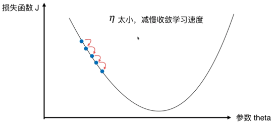
• $\eta$ 称为学习率（Learning Rate）
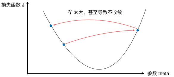
• $\eta$ 的取值影响获得最优解的速度
• $\eta$ 取值不合适甚至得不到最优解
• $\eta$ 是梯度下降算法的一个超参数
  
  

1.3 代码实现梯度下降算法

import numpy as np
import matplotlib.pyplot as plt
plot_x = np.linspace(-1,6,141)
# print(plot_x)
plot_y = (plot_x - 2.5) ** 2 -1

plt.plot(plot_x,plot_y)
# plt.show()

def dJ(theta):
    return 2 * (theta - 2.5)
def J(theta):
    return (theta - 2.5) ** 2 -1

theta = 0.0
eta = 0.1
epsilon = 1e-8
theta_history = [theta]
while True:
    gradieent = dJ(theta)
    last_theta = theta
    theta = theta - eta * gradieent
    theta_history.append(theta)

    if(abs(J(theta) -J(last_theta)) < epsilon):
        break

plt.plot(np.array(theta_history), J(np.array(theta_history)), color = 'r', marker = '+')
plt.show()

print(theta)
print(J(theta))
#**************************运行结果***************************************
#                      2.499891109642585
#                     -0.99999998814289

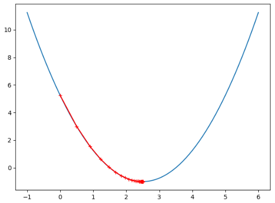
显然我们实现的梯度下降算法已经达到了我们想要的效果，下面我们对上面的代码进行封装，再看看不同的 $\theta$ 取值对算法效果的影响：

import numpy as np
import matplotlib.pyplot as plt
plot_x = np.linspace(-1,6,141)

def dJ(theta):
    return 2 * (theta - 2.5)

def J(theta):
    return (theta - 2.5) ** 2 -1

def gradient_descent(initial_theta, eta, epsilon=1e-8):
    theta = initial_theta
    theta_history.append(initial_theta)
    while True:
        gradieent = dJ(theta)
        last_theta = theta
        theta = theta - eta * gradieent
        theta_history.append(theta)

        if (abs(J(theta) - J(last_theta)) < epsilon):
            break

def plot_theta_history():
    plt.plot(plot_x, J(plot_x))
    plt.plot(np.array(theta_history), J(np.array(theta_history)), color='r', marker='+')
    plt.show()

eta = 0.01
theta_history = []
gradient_descent(0.0, eta)
plot_theta_history()
#***************************************运行结果************************
#            如下图

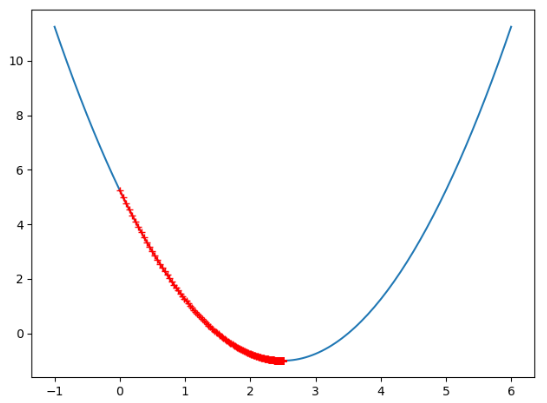
相比我们将 $\theta$ 设置为0.1，此时的 $\theta = 0.01$ 显然此时已经近乎拟合了曲线。如果我们把 $\theta$ 的取值设置的更大一点呢？

eta = 0.8
theta_history = []
gradient_descent(0.0, eta)
plot_theta_history()

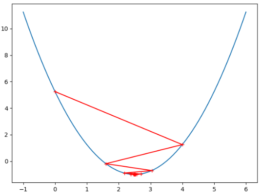
虽然此时我们的梯度下降算法并没有很好的拟合我们的曲线，但是依然有效，依旧找到了最优解，因此我们知道， $\theta$ 的值只要不超过某个限定的值就是有效的。
下面我们试着将 $\theta$ 的值设置为1.1
此时编译器直接报错

OverflowError: (34, 'Result too large')

此时因为我们选取的 $\eta$ 值过大，是的我们无法求得最优解，我我们修改一下代码，用matplot画出直观的图示来看看究竟发生了什么。
首先我们将gradient_descent函数中添加一个n_iterations变量来控制循环次数，再改变while循环的条件

ef gradient_descent(initial_theta,eta, n_iterations = 1e4,  epsilon=1e-8):
    theta = initial_theta
    theta_history.append(initial_theta)
    i_iter = 0
    while i_iter < n_iterations:
        gradieent = dJ(theta)
        last_theta = theta
        theta = theta - eta * gradieent
        theta_history.append(theta)

        if (abs(J(theta) - J(last_theta)) < epsilon):
            break
        i_iter += 1

我们让while循环执行10次查看结果

eta = 1.1
theta_history = []
gradient_descent(0.0,  eta,n_iterations=10)
plot_theta_history()

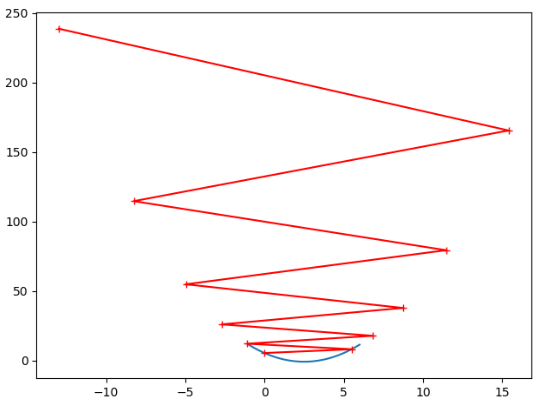
从结果中我们可以明显看到， $\theta$ 取值过大， $J(\theta)$ 的值也随之越来越大，而且我们这里只循环了10次，在之前我们的while循环直接等于true，一直在死循环，所以才会报OverflowError: (34, 'Result too large')的错误！

2 多元线性回归中的梯度下降算法

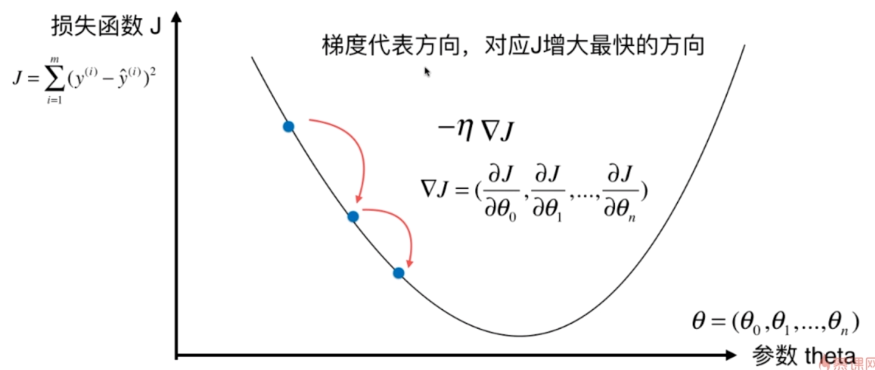
在参数只有一个的情况下，我们知道斜率对应于 $J$ 增大的方向，而在多个参数的情况下梯度 $\nabla J$ 表示 $J$增大最快的方向
在之前的多元线性回归算法中我们的目标函数为
$\sum_{i=1}^m{(y^{(i)}-\hat{y}^{(i)})^2}$
$\hat{y}^{(i)}=\theta_0+\theta_0x_1^{(i)}+\theta_0x_2^{(i)}+\cdots+\theta_0x_n^{(i)}$
所以也就是求
$\sum_{i=1}^m{(y^{(i)}-\theta_0-\theta_0x_1^{(i)}-\theta_0x_2^{(i)}-\cdots-\theta_0x_n^{(i)})^2}$
尽可能小。
下面我们来求这一函数的梯度：
$\nabla J= \begin{pmatrix} \frac{\partial J}{\partial \theta_0} \\ \frac{\partial J}{\partial \theta_1} \\ \frac{\partial J}{\partial \theta_2} \\ \vdots \\ \frac{\partial J}{\partial \theta_n} \end{pmatrix}= \begin{pmatrix} \sum_{i=1}^m2(y^{(i)}-X_b^{(i)}\theta)·(-1) \\ \sum_{i=1}^m2(y^{(i)}-X_b^{(i)}\theta)·(-X_1^{(i)}) \\ \sum_{i=1}^m2(y^{(i)}-X_b^{(i)}\theta)·(-X_2^{(i)}) \\ \vdots \\ \sum_{i=1}^m2(y^{(i)}-X_b^{(i)}\theta)·(-X_n^{(i)}) \end{pmatrix}$

$=2 \begin{pmatrix} \sum_{i=1}^m(X_b^{(i)}\theta-y^{(i)})· \\ \sum_{i=1}^m(X_b^{(i)}\theta-y^{(i)})·X_1^{(i)} \\ \sum_{i=1}^m(X_b^{(i)}\theta-y^{(i)})·X_2^{(i)} \\ \vdots \\ \sum_{i=1}^m(X_b^{(i)}\theta-y^{(i)})·X_n^{(i)} \end{pmatrix}$
观察发现这个式子于 $m$ 相关，也就是说于样本的数量相关，如果样本数量越大，那么梯度中的元素值越大，显然这并不是我们想要的结果，为了消去 $m$ 的影响，我们把结果除以 $m$ 即：
$\frac{2}{m} \begin{pmatrix} \sum_{i=1}^m(X_b^{(i)}\theta-y^{(i)})· \\ \sum_{i=1}^m(X_b^{(i)}\theta-y^{(i)})·X_1^{(i)} \\ \sum_{i=1}^m(X_b^{(i)}\theta-y^{(i)})·X_2^{(i)} \\ \vdots \\ \sum_{i=1}^m(X_b^{(i)}\theta-y^{(i)})·X_n^{(i)} \end{pmatrix}$
此时的目标函数也相应得改为：
$\frac{1}{m}\sum_{i=1}^m{(y^{(i)}-\hat{y}^{(i)})^2}$
这个式子我们应该很熟悉就是前面所学的 $MSE$ 也即
$J(\theta) = MSE(y,\hat{y})$
有时我们也取
$J(\theta) =\frac{1}{2m}\sum_{i=1}^m{(y^{(i)}-\hat{y}^{(i)})^2}$
来消去梯度中计算结果中的2，但是两者一般情况下并没有什么显著的差距。

2.1 实现多元线性回归中的梯度下降算法

我们在之前的多元线性回归算法中封装了一个fit_nomal的方法，现在我们使用同样的方法封装一个fit_gd的方法，以后使用时直接调用这个方法即可

 def fit_gd(self,X_train,y_train,eta=0.01,n_iterations=1e4):
        """根据训练数据集X_train训练 Linear Regression模型"""
        assert X_train.shape[0] == y_train.shape[0], \
            "the size of X_train must be equal to the size of y_train"

        def J(theta, x_b, y):
            try:
                return np.sum((y - x_b.dot(theta)) ** 2) / len(x_b)
            except:
                return float('inf')

        def dJ(theta, x_b, y):
            res = np.empty(len(theta))
            res[0] = np.sum(x_b.dot(theta) - y)
            for i in range(1, len(theta)):
                res[i] = (x_b.dot(theta) - y).dot(x_b[:, i])
            return res * 2 / len(x_b)


        def gradient_descent(x_b, y, initial_theta, eta, n_iterations=1e4, epsilon=1e-8):
            theta = initial_theta
            i_iter = 0
            while i_iter < n_iterations:
                gradient = dJ(theta, x_b, y)
                last_theta = theta
                theta = theta - eta * gradient

                if (abs(J(theta, x_b, y) - J(last_theta, x_b, y)) < epsilon):
                    break
                i_iter += 1
            return theta
        x_b = np.hstack([np.ones((len(X_train), 1)), X_train])
        initial_theta = np.zeros(x_b.shape[1])
        self._theta=gradient_descent(x_b,y_train,initial_theta,eta,n_iterations)
        self.interception_=self._theta[0]
        self.coef_ = self._theta[1:]

这样就将这个fit_gd方法封装进了LinearRegression这个类当中了，我们看一下具体怎么使用

import numpy as np
import matplotlib.pyplot as plt
from LinearRegression import LinearRegression
lin_reg = LinearRegression()
np.random.seed(666)
x = np.random.random(size=100)
y = x * 3. + 4. + np.random.normal(size=100)
X = x.reshape(-1,1)
lin_reg.fit_gd(X,y)
print(lin_reg.coef_)
print(lin_reg.interception_)
#***************运行结果********************
#                [3.0043078]
#                4.0269033037832385

可以看到运行的结果符合我们模拟的直线 $y=3x+4$

To Be Continued