梯度下降是一种优化算法,用于最小化各种机器学习算法中的成本函数。它主要用于更新学习模型的参数。
梯度下降的类型:
- 批量梯度下降:
这是一种梯度下降,它为梯度下降的每次迭代处理所有训练示例。但是如果训练样本的数量很大,那么批量梯度下降在计算上是非常昂贵的。因此,如果训练示例的数量很大,那么批量梯度下降不是首选。相反,我们更喜欢使用随机梯度下降或小批量梯度下降。 - 随机梯度下降:
这是一种梯度下降,每次迭代处理一个训练示例。因此,即使在仅处理了一个示例的一次迭代之后,参数也会被更新。因此,这比批量梯度下降要快得多。但是同样,当训练示例的数量很大时,即使这样它也只处理一个示例,这可能会给系统带来额外的开销,因为迭代次数会非常大。 - 小批量梯度下降:
这是一种比批量梯度下降和随机梯度下降更快的梯度下降。这里b个示例,其中b<m是每次迭代处理的。所以即使训练样例的数量很大,也可以一次性批量处理b个训练样例。因此,它适用于更大的训练示例,并且迭代次数也更少。
使用的变量:
设 m 为训练示例的数量。
设 n 为特征数。
注意:
如果 b == m,那么小批量梯度下降的行为类似于批量梯度下降。
1.批量梯度下降算法:
假设 h θ (x) 是线性回归的假设。然后,成本函数由下式给出:
令 Σ 表示从 i=1 到 m 的所有训练示例的总和。
Jtrain(θ) = (1/2m) Σ( hθ(x(i))  - y(i))2

Repeat {


 θj = θj – (learning rate/m) * Σ( hθ(x(i))  - y(i))xj(i)
    For every j =0 …n
}
其中 x j (i)表示第 i个训练样例的第 j个特征。所以如果m非常大(例如 500 万个训练样本),那么需要几个小时甚至几天才能收敛到全局最小值。这就是为什么对于大型数据集,不建议使用批量梯度下降,因为它会减慢学习速度。
2.随机梯度下降算法SGD:
1)随机打乱数据集,以便对每种类型的数据均匀地训练参数。
2)如上所述,每次迭代考虑一个示例。
Hence,
Let (x(i),y(i)) be the training example
Cost(θ, (x(i),y(i))) = (1/2) Σ( hθ(x(i))  - y(i))2

Jtrain(θ) = (1/m) Σ Cost(θ, (x(i),y(i)))

Repeat {


For i=1 to m{


         θj = θj – (learning rate) * Σ( hθ(x(i))  - y(i))xj(i)
        For every j =0 …n

                }
}
在 SGD 中,我们在每次迭代中找出单个示例的成本函数的梯度,而不是所有示例的成本函数的梯度之和。
在 SGD 中,由于每次迭代仅从数据集中随机选择一个样本,因此算法达到最小值所采用的路径通常比典型的梯度下降算法更嘈杂。但这并不重要,因为算法所采用的路径并不重要,只要我们达到最小值并且训练时间显着缩短。
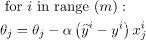
Batch Gradient Descent 采用的路径——

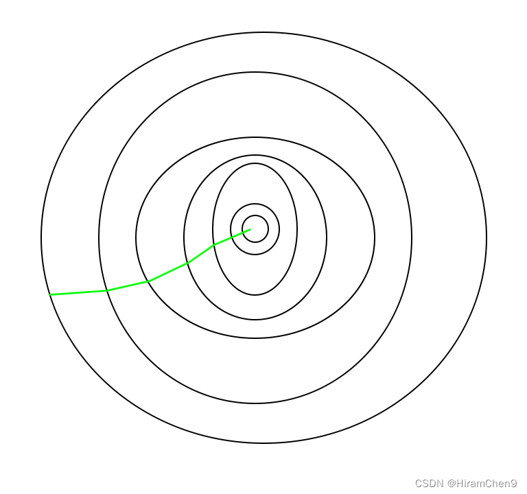
随机梯度下降已经采取了一条路径——
需要注意的一件事是,由于 SGD 通常比典型的梯度下降更嘈杂,因此通常需要更多的迭代次数才能达到最小值,因为它在下降过程中具有随机性。尽管它比典型的梯度下降需要更多的迭代次数才能达到最小值,但它在计算上仍然比典型的梯度下降便宜得多。因此,在大多数情况下,SGD 优于批量梯度下降来优化学习算法。
Python 中 SGD 的伪代码:
def SGD(f, theta0, alpha, num_iters):
	"""
	Arguments:
	f -- the function to optimize, it takes a single argument
			and yield two outputs, a cost and the gradient
			with respect to the arguments
	theta0 -- the initial point to start SGD from
	num_iters -- total iterations to run SGD for
	Return:
	theta -- the parameter value after SGD finishes
	"""
	start_iter = 0
	theta = theta0
	for iter in xrange(start_iter + 1, num_iters + 1):
		_, grad = f(theta)

		# there is NO dot product ! return theta
		theta = theta - (alpha * grad)
3.小批量梯度下降算法:
假设 b 是一批中的示例数,其中 b < m。
假设b = 10,m = 100;
注意:
但是我们可以调整批量大小。它通常保持为 2 的幂。其背后的原因是因为某些硬件(例如 GPU)通过常见的批量大小(例如 2 的幂)实现了更好的运行时间。
Repeat {


 For i=1,11, 21,…..,91

    Let Σ be the summation from i to i+9 represented by k.

    θj = θj – (learning rate/size of (b) ) * Σ( hθ(x(k))  - y(k))xj(k)
        For every j =0 …n

}
梯度下降不同变体的收敛趋势:
在批量梯度下降的情况下,算法沿着一条直线走向最小值。如果成本函数是凸的,那么它会收敛到全局最小值,如果成本函数不是凸的,那么它会收敛到局部最小值。这里学习率通常保持不变。
在随机梯度下降和小批量梯度下降的情况下,算法不会收敛,而是继续在全局最小值附近波动。因此,为了使其收敛,我们必须慢慢改变学习率。然而,随机梯度下降的收敛噪声更大,因为在一次迭代中,它只处理一个训练样本。
Python实现:
第 1 步:
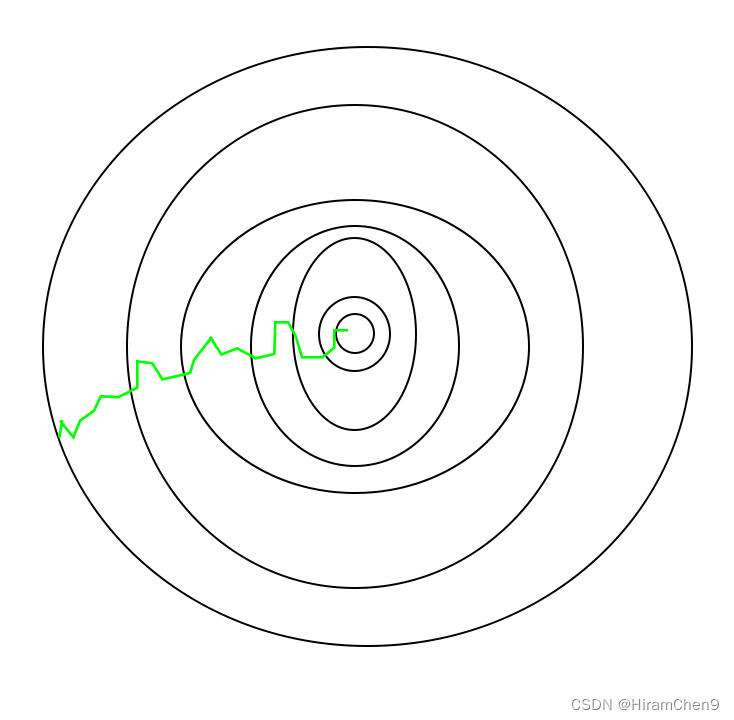
第一步是导入依赖项,为线性回归生成数据,并可视化生成的数据。我们已经生成了 8000 个数据示例,每个示例都有 2 个属性/特征。这些数据样本进一步分为训练集(X_train,y_train)和测试集(X_test,y_test),分别有7200和800个样本。
# importing dependencies
import numpy as np
import matplotlib.pyplot as plt

# creating data
mean = np.array([5.0, 6.0])
cov = np.array([[1.0, 0.95], [0.95, 1.2]])
data = np.random.multivariate_normal(mean, cov, 8000)

# visualising data
plt.scatter(data[:500, 0], data[:500, 1], marker='.')
plt.show()

# train-test-split
data = np.hstack((np.ones((data.shape[0], 1)), data))

split_factor = 0.90
split = int(split_factor * data.shape[0])

X_train = data[:split, :-1]
y_train = data[:split, -1].reshape((-1, 1))
X_test = data[split:, :-1]
y_test = data[split:, -1].reshape((-1, 1))

print(& quot
	Number of examples in training set= % d & quot
	% (X_train.shape[0]))
print(& quot
	Number of examples in testing set= % d & quot
	% (X_test.shape[0]))
输出:
训练集中的示例数 = 7200 测试集中的示例数 = 800
第二步:
接下来,我们编写使用小批量梯度下降实现线性回归的代码。gradientDescent() 是主要的驱动函数,其他函数是辅助函数,用于进行预测——hypothesis()、计算梯度——gradient()、计算误差——cost() 和创建小批量——create_mini_batches()。驱动程序函数初始化参数,计算模型的最佳参数集,并返回这些参数以及一个列表,其中包含参数更新时的错误历史记录。
例子
# linear regression using "mini-batch" gradient descent
# function to compute hypothesis / predictions


def hypothesis(X, theta):
	return np.dot(X, theta)

# function to compute gradient of error function w.r.t. theta


def gradient(X, y, theta):
	h = hypothesis(X, theta)
	grad = np.dot(X.transpose(), (h - y))
	return grad

# function to compute the error for current values of theta


def cost(X, y, theta):
	h = hypothesis(X, theta)
	J = np.dot((h - y).transpose(), (h - y))
	J /= 2
	return J[0]

# function to create a list containing mini-batches


def create_mini_batches(X, y, batch_size):
	mini_batches = []
	data = np.hstack((X, y))
	np.random.shuffle(data)
	n_minibatches = data.shape[0] // batch_size
	i = 0

	for i in range(n_minibatches + 1):
		mini_batch = data[i * batch_size:(i + 1)*batch_size, :]
		X_mini = mini_batch[:, :-1]
		Y_mini = mini_batch[:, -1].reshape((-1, 1))
		mini_batches.append((X_mini, Y_mini))
	if data.shape[0] % batch_size != 0:
		mini_batch = data[i * batch_size:data.shape[0]]
		X_mini = mini_batch[:, :-1]
		Y_mini = mini_batch[:, -1].reshape((-1, 1))
		mini_batches.append((X_mini, Y_mini))
	return mini_batches

# function to perform mini-batch gradient descent


def gradientDescent(X, y, learning_rate=0.001, batch_size=32):
	theta = np.zeros((X.shape[1], 1))
	error_list = []
	max_iters = 3
	for itr in range(max_iters):
		mini_batches = create_mini_batches(X, y, batch_size)
		for mini_batch in mini_batches:
			X_mini, y_mini = mini_batch
			theta = theta - learning_rate * gradient(X_mini, y_mini, theta)
			error_list.append(cost(X_mini, y_mini, theta))

	return theta, error_list
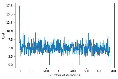
调用 gradientDescent() 函数来计算模型参数 (theta) 并可视化误差函数的变化。
theta, error_list = gradientDescent(X_train, y_train)
print("Bias = ", theta[0])
print("Coefficients = ", theta[1:])

# visualising gradient descent
plt.plot(error_list)
plt.xlabel("Number of iterations")
plt.ylabel("Cost")
plt.show()
输出:
偏差 = [0.81830471] 系数 = [[1.04586595]]
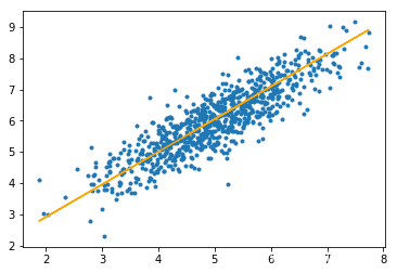
第三步:
最后,我们对测试集进行预测并计算预测中的平均绝对误差。
# predicting output for X_test
y_pred = hypothesis(X_test, theta)
plt.scatter(X_test[:, 1], y_test[:, ], marker='.')
plt.plot(X_test[:, 1], y_pred, color='orange')
plt.show()

# calculating error in predictions
error = np.sum(np.abs(y_test - y_pred) / y_test.shape[0])
print(& quot
	Mean absolute error = & quot
	, error)
输出:
平均绝对误差 = 0.4366644295854125
橙色线代表最终假设函数:theta[0] + theta[1]*X_test[:, 1] + theta[2]*X_test[:, 2] = 0
the end.