神经网络优化----正则化 （正则化损失函数）

在神经网络优化中，通过对损失函数进行正则化来缓解过拟合

方法：通过在损失函数中引入模型复杂度指标，利用给W加权值，弱化了训练数据的噪声

公式为：

loss = loss(y与y_) + regularizer * loss(w)

其中 loss(y与y_)为一般损失函数，可以为交叉熵损失函数，或者均方误差损失函数

regularizer为正则化权重

regularizer * loss(w) 在python中用一下代码实现：

tf.contrib.layers.l2_regularizer(regularizer)(w)

下面是全部代码及运行截图

#coding:utf-8
import tensorflow as tf
import numpy as np
import matplotlib.pyplot as plt #引入图形可视化工具

#正则化损失函数
#loss = loss(y与y_) + regularizer * loss(w) 此为正则化损失函数

BATCH_SIZE = 30 #批处理量，一次神经网络训练量

#基于seed产生随机数
seed = 2
rdm = np.random.RandomState(seed)

#将随机数输入300行2列的矩阵，作为输入数据集
X = rdm.randn(300,2)

#从输入数据集矩阵依次取出每行（x0,x1）,若 x0*x0 + x1*x1 <2 ,则将 Y_ 赋值为1 ，否则赋值为0
Y_ = [int(x0*x0 + x1*x1 <2 ) for (x0,x1) in X]

#根据 Y_ 的值给出颜色，若为1，赋值为红色，否则赋值为蓝色
Y_c = [['red' if y else 'blue'] for y in Y_]

#对 X 和 Y_ 的形状进行整理，将 X 变成 n 行 2 列的矩阵，将 Y_ 整理成 n 行 1 列的矩阵，其中 n 用 -1 表示
X = np.vstack(X).reshape(-1,2)
Y_ = np.vstack(Y_).reshape(-1,1)

#将 X , Y_ , Y_c 打印出来
print(X)
print(Y_)
print(Y_c)

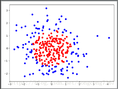
#用plt.scatter画出数据集X各行中的第0列和第1列元素组成的点（x0，x1），用Y_c对点进行着色（c代表color）
plt.scatter(X[:,0],X[:,1],c = np.squeeze(Y_c))
plt.show()

#loss = loss(y与y_) + regularizer * loss(w) 此为正则化损失函数
# regularizer * loss(w) 可用 tf.contrib.layers.l2_regularizer(regularizer)(w) 实现
def get_weight(shape,regularizer): #shape为列表，regularizer为正则化权重
    w = tf.Variable(tf.random_normal(shape),dtype=tf.float32)
    tf.add_to_collection('losses',tf.contrib.layers.l2_regularizer(regularizer)(w)) #正则化，来缓解过拟合,将所有计算好的正则化了的 w 加在 losses 赋值在上
    return w


def get_bias(shape):
    b = tf.Variable(tf.constant(0.01,shape=shape)) #初始化赋值为0.01，用shape传入参数赋值给b
    return b

x = tf.placeholder(tf.float32,shape=(None,2))
y_ = tf.placeholder(tf.float32,shape=(None,1))

#第一层神经网络
w1 = get_weight([2,11],0.01)
b1 = get_bias([11])
y1 = tf.nn.relu(tf.matmul(x,w1)+b1) #relu激活函数，除了输出层一定用sigmoid激活函数外，其它层基本都用relu激活函数

#第二层神经网络，输出层
w2 = get_weight([11,1],0.01)
b2 = get_bias([1])
y = tf.matmul(y1,w2)+b2 #输出层不用激活

#损失函数
loss_mse = tf.reduce_mean(tf.square(y-y_)) #均方误差损失函数，此为原始损失函数 loss(y与y_)
#loss = loss(y与y_) + regularizer * loss(w) 此为正则化损失函数
loss_total = loss_mse + tf.add_n(tf.get_collection('losses')) #将均方误差损失函数和正则化了的所有的 w 的和的值相加得到更有效的损失函数

#训练方法，用不同的损失函数，效果不同，正则化了的损失函数效果更好
train_step = tf.train.AdamOptimizer(0.001).minimize(loss_mse)
#train_step = tf.train.AdamOptimizer(0.001).minimize(loss_total)

#生成会话，开始训练
with tf.Session() as sess:
    #初始化所有参数
    init_op = tf.global_variables_initializer()
    sess.run(init_op)
    STEPS = 40000  #训练轮数
    for i in range(STEPS):
        start = (i*BATCH_SIZE)%300
        end = start + BATCH_SIZE
        sess.run(train_step,feed_dict={x:X[start:end],y_:Y_[start:end]})  #喂入数据，开始训练
        if i % 2000 == 0:
            loss_mse_v = sess.run(loss_mse,feed_dict={x:X,y_:Y_})
            print("Aftre %d steps ,the loss is %f"%(i,loss_mse_v))

    xx ,yy = np.mgrid[-3:3:.01 ,-3:3:.01] #np.mgrid[起：止：步长，起：止：步长]  表示x轴，y轴的起点，终点，两点之间的步长
    grid = np.c_[xx.ravel(),yy.ravel()]  #通过eavel()函数将xx,yy拉直，并通过np.c_上述xx,yy组成矩阵，形成网格坐标点

    probs = sess.run(y,feed_dict={x:grid}) #将所有的网格坐标点喂入神经网络，经神经网络计算推测得出结果y，将y赋值给probs ，此probs为所有红色点或者蓝色点的量化值
    probs = probs.reshape(xx.shape) #将probs整理为xx的矩阵的形状
    print("")
    print("w1:",sess.run(w1))
    print("b1：",sess.run(b1))
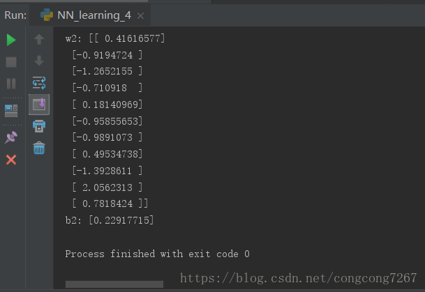
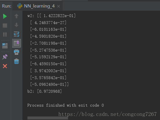
    print("w2:",sess.run(w2))
    print("b2:",sess.run(b2))


plt.scatter(X[:,0],X[:,1],c = np.squeeze(Y_c))
plt.contour(xx,yy,probs,levels=[.5]) #plt.contour(x轴坐标值，y轴坐标值，该点的高度，levels=[等高线的高度]) 通过x轴坐标，y轴坐标和各点的高度，将指定高度的点描上颜色
plt.show()

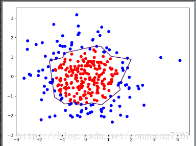
运行截图

下面是损失函数为loss_mse是的截图

下面是损失函数为loss_total的运行截图

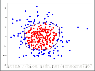
可以有图像直观看出来，正则化了的损失函数效果更好