import pandas as pd
import pylab
import math
import numpy as np
import matplotlib.pyplot as plt
%matplotlib inline
from scipy.stats import norm
import scipy.stats
import warnings
warnings.filterwarnings("ignore")

df=pd.read_csv("http://ww2.amstat.org/publications/jse/datasets/normtemp.dat.txt",sep="   ",names=['Temperature','Gender','Heart Rate'])
df.head()
| |
Temperature |
Gender |
Heart Rate |
| 0 |
96.3 |
1 |
70 |
| 1 |
96.7 |
1 |
71 |
| 2 |
96.9 |
1 |
74 |
| 3 |
97.0 |
1 |
80 |
| 4 |
97.1 |
1 |
73 |
df.describe()
| |
Temperature |
Gender |
Heart Rate |
| count |
130.000000 |
130.000000 |
130.000000 |
| mean |
98.249231 |
1.500000 |
73.761538 |
| std |
0.733183 |
0.501934 |
7.062077 |
| min |
96.300000 |
1.000000 |
57.000000 |
| 25% |
97.800000 |
1.000000 |
69.000000 |
| 50% |
98.300000 |
1.500000 |
74.000000 |
| 75% |
98.700000 |
2.000000 |
79.000000 |
| max |
100.800000 |
2.000000 |
89.000000 |
#假设检验
#前提检验正态分布
observed_temperatures = df['Temperature'].sort_values()
bin_val = np.arange(start = observed_temperatures.min(),stop=observed_temperatures.max(),step=50)
mu,std = np.mean(observed_temperatures),np.std(observed_temperatures)

p = norm.pdf(observed_temperatures, mu,std)

plt.hist(observed_temperatures,bins=bin_val,normed=True,stacked=True)
plt.plot(observed_temperatures,p,color='r')
plt.xticks(np.arange(95.75,101.25,0.25),rotation=90)
plt.xlabel('Human Body Temperature Distributions')
plt.ylabel('human body temperature')
plt.show()
print("Average (Mu):"+str(mu)+"/ Standard Deviation:" + str(std))
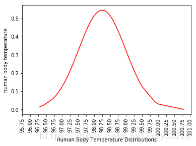
Average (Mu):98.24923076923076/ Standard Deviation:0.7303577789050376
#确定指标进行正态检验
x = observed_temperatures
shapiro_test,shapiro_p = scipy.stats.shapiro(x)
print("Shapiro-Wilk Stat:",shapiro_test,"Shapiro-Wilk p-Value:",shapiro_p)
k2,p = scipy.stats.normaltest(observed_temperatures)
print("k2:",k2,"p:",p)
#以上两种方法,p值大于0.05,认为正态分布
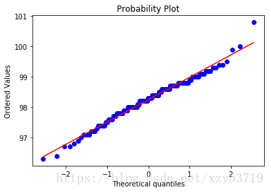
#Another method to determining normality is through Quantile-Quantile Plots
#QQ图检查正态分布
scipy.stats.probplot(observed_temperatures,dist='norm',plot=pylab)
pylab.show()
Shapiro-Wilk Stat: 0.9865769743919373 Shapiro-Wilk p-Value: 0.2331680953502655
k2: 2.703801433319236 p: 0.2587479863488212
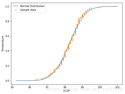
#另一种检测正态分布的方法
def ecdf(data):
    #Compute ECDF
    n = len(data)
    x = np.sort(data)
    y = np.arange(1,n+1) / n
    return x,y
# Compute empirical mean and standard deviation

#Number of samples
n = len(df['Temperature'])

#Sample mean
mu = np.mean(df['Temperature'])

#Sample standard deviation
std = np.std(df['Temperature'])

print("Mean Temperature:",mu,"Standard deviation:",std)

#基于当前的均值和标准差,随机生成一个正态分布
normalized_sample = np.random.normal(mu,std,size=10000)
normalized_x,normalized_y = ecdf(normalized_sample)

x_temperature,y_temperature = ecdf(df['Temperature'])

#Plot the ECDFs
fig = plt.figure(figsize=(8,6))
plt.plot(normalized_x,normalized_y)
plt.plot(x_temperature,y_temperature,marker='.',linestyle='none')
plt.xlabel('ECDF')
plt.ylabel("Temperature")
plt.legend(("Normal Distribution","Sample data"))
Mean Temperature: 98.24923076923076 Standard deviation: 0.730357778905038
Out[73]:
<matplotlib.legend.Legend at 0xb3437b8>
#验证98.6为平均温度
from scipy import stats
CW_mu = 98.6
stats.ttest_1samp(df['Temperature'],CW_mu,axis=0)
#T-Stat -5.454 p-value 近乎0,拒绝原假设
Ttest_1sampResult(statistic=-5.454823292364077, pvalue=2.410632041561008e-07)
#检验男女体温是否明显区别
#两独立样本t检验
#H0:两样本没有明显差异,H1:有明显差异
female_temperature = df.Temperature[df.Gender==2]
male_temperature = df.Temperature[df.Gender==1]
mean_female_temperature = female_temperature.mean()
mean_male_temperature = male_temperature.mean()
print("男体温均值:",mean_male_temperature,"女体温均值:",mean_female_temperature)

#两独立样本t检验
stats.ttest_ind(female_temperature,male_temperature,axis=0)

#由于p值0.024 < 0.05 ,拒绝原假设,我们有95%的自信度认为是有差异的
男体温均值: 98.1046153846154 女体温均值: 98.39384615384616
Ttest_indResult(statistic=2.2854345381654984, pvalue=0.02393188312240236)