数据集:数据集采用Sort_1000pics数据集。数据集包含1000张图片,总共分为10类。分别是人(0),沙滩(1),建筑(2),大卡车(3),恐龙(4),大象(5),花朵(6),马(7),山峰(8),食品(9)十类,每类100张,(数据集可以到网上下载)。
ubuntu16.04虚拟操作系统,在分配内存4G,处理器为1个CPU下的环境下运行。
将所得到的图片至“./photo目录下”,(这里采用的是Anaconda3作为开发环境)。可以参考上一篇
伯努利分布理论基础:
该分布研究的是一种特殊的实验,这种实验只有两个结果要么成功要么失败,且每次实验是独立的并每次实验都有固定的成功概率p。用伯努利朴素贝叶斯实现对图像的分类,首先伯努利分类对象是0,1分类,故此需要将图像像素进行阈值0,1划分。


import datetime
starttime = datetime.datetime.now()
import numpy as np
from sklearn.cross_validation import train_test_split
from sklearn.metrics import confusion_matrix, classification_report
import os
import cv2
X = []
Y = []
for i in range(0, 10):
#遍历文件夹,读取图片
for f in os.listdir("./photo/%s" % i):
#打开一张图片并灰度化
Images = cv2.imread("./photo/%s/%s" % (i, f))
image=cv2.resize(Images,(256,256),interpolation=cv2.INTER_CUBIC)
hist = cv2.calcHist([image], [0,1], None, [256,256], [0.0,255.0,0.0,255.0])
X.append(((hist/255).flatten()))
Y.append(i)
X = np.array(X)
Y = np.array(Y)
#切分训练集和测试集
X_train, X_test, y_train, y_test = train_test_split(X, Y, test_size=0.3, random_state=1)
#随机率为100%(保证唯一性可以对比)选取其中的30%作为测试集
from sklearn.preprocessing import binarize
from sklearn.preprocessing import LabelBinarizer
class ML:
def predict(self, x):
#预测标签
X = binarize(x, threshold=self.threshold)
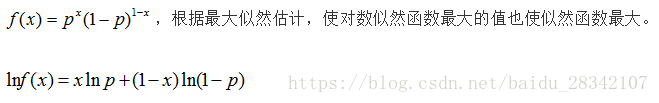
#使对数似然函数最大的值也使似然函数最大
#Y_predict = np.dot(X, np.log(prob).T)+np.dot(np.ones((1,prob.shape[1]))-X, np.log(1-prob).T)
#等价于 lnf(x)=xlnp+(1-x)ln(1-p)
Y_predict = np.dot(X, np.log(self.prob).T)-np.dot(X, np.log(1-self.prob).T) + np.log(1-self.prob).sum(axis=1)
return self.classes[np.argmax(Y_predict, axis=1)]
class Bayes(ML):
def __init__(self,threshold):
self.threshold = threshold
self.classes = []
self.prob = 0.0
def fit(self, X, y):
#标签二值化
labelbin = LabelBinarizer()
Y = labelbin.fit_transform(y)
self.classes = labelbin.classes_ #统计总的类别,10类
Y = Y.astype(np.float64)
#转换成二分类问题
X = binarize(X, threshold=self.threshold)#特征二值化,threshold阈值根据自己的需要适当修改
feature_count = np.dot(Y.T, X) #矩阵转置,对相同特征进行融合
class_count = Y.sum(axis=0) #统计每一类别出现的个数
#拉普拉斯平滑处理,解决零概率的问题
alpha = 1.0
smoothed_fc = feature_count + alpha
smoothed_cc = class_count + alpha * 2
self.prob = smoothed_fc/smoothed_cc.reshape(-1, 1)
return self
clf0 = Bayes(0.2).fit(X_train,y_train) #0.2表示阈值
predictions_labels = clf0.predict(X_test)
print(confusion_matrix(y_test, predictions_labels))
print (classification_report(y_test, predictions_labels))
endtime = datetime.datetime.now()
print (endtime - starttime)
实验结果为:
[[20  0  0  0  0  1  0 10  0  0]
 [ 1  2  5  0  0  0  0 23  0  0]
 [ 3  0  9  0  1  0  0 13  0  0]
 [ 0  0  1 18  0  1  1  5  0  3]
 [ 0  0  0  0 30  1  0  0  0  1]
 [ 0  0  0  0  1  6  0 26  0  1]
 [ 3  0  0  2  0  0 21  3  0  1]
 [ 0  0  0  0  0  0  0 26  0  0]
 [ 2  0  0  2  1  1  0 21  2  2]
 [ 2  0  2  3  1  0  1 15  0  6]]
             precision    recall  f1-score   support

          0       0.65      0.65      0.65        31
          1       1.00      0.06      0.12        31
          2       0.53      0.35      0.42        26
          3       0.72      0.62      0.67        29
          4       0.88      0.94      0.91        32
          5       0.60      0.18      0.27        34
          6       0.91      0.70      0.79        30
          7       0.18      1.00      0.31        26
          8       1.00      0.06      0.12        31
          9       0.43      0.20      0.27        30

avg / total       0.70      0.47      0.45       300

0:00:05.261369
大家可根据自己的数据集图像,调整划分阈值,可以得到不同的分类精度。代码参考了from sklearn.naive_bayes import BernoulliNB里面的代码。下面贴出集成的代码:
import datetime
starttime = datetime.datetime.now()

import numpy as np
from sklearn.cross_validation import train_test_split
from sklearn.metrics import confusion_matrix, classification_report
import os
import cv2

X = []
Y = []

for i in range(0, 10):
    #遍历文件夹,读取图片
    for f in os.listdir("./photo/%s" % i):
        #打开一张图片并灰度化
        Images = cv2.imread("./photo/%s/%s" % (i, f))
        image=cv2.resize(Images,(256,256),interpolation=cv2.INTER_CUBIC)
        hist = cv2.calcHist([image], [0,1], None, [256,256], [0.0,255.0,0.0,255.0])
        X.append(((hist/255).flatten()))
        Y.append(i)
X = np.array(X)
Y = np.array(Y)
#切分训练集和测试集
X_train, X_test, y_train, y_test = train_test_split(X, Y, test_size=0.3, random_state=1)

from sklearn.naive_bayes import BernoulliNB
clf0 = BernoulliNB().fit(X_train, y_train)
predictions0 = clf0.predict(X_test)
print (classification_report(y_test, predictions0))
endtime = datetime.datetime.now()
print (endtime - starttime)
precision    recall  f1-score   support

          0       0.52      0.42      0.46        31
          1       0.48      0.52      0.50        31
          2       0.39      0.54      0.45        26
          3       0.63      0.59      0.61        29
          4       0.76      0.88      0.81        32
          5       0.58      0.41      0.48        34
          6       0.94      0.53      0.68        30
          7       0.51      0.69      0.59        26
          8       0.47      0.52      0.49        31
          9       0.75      0.80      0.77        30

avg / total       0.61      0.59      0.59       300

0:00:05.426743