Logistic Regression
上一次的课程主要解决回归分析问题,这一次的课程主要为分类问题,分类问题也可看做将回归问题的连续性离散化。
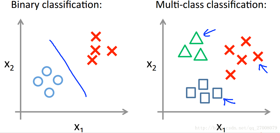
1.1 Classification
先来谈谈二分类问题。课程中先给出了几个例子。

邮件是垃圾邮件还是非垃圾邮件;网上交易是的欺骗性(Y or N);肿瘤是恶性的还是良性的。
对于这些问题,我们可以通过输出值y
通过上次的课程,我们可以想到利用假设函数
1.2 Hypothesis Representation
Sigmoid function:
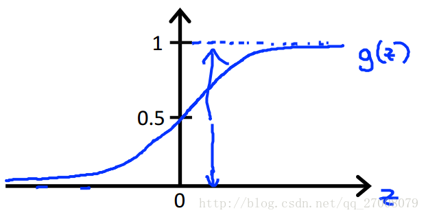
假设函数代表了一种概率含义
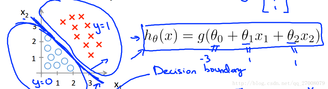
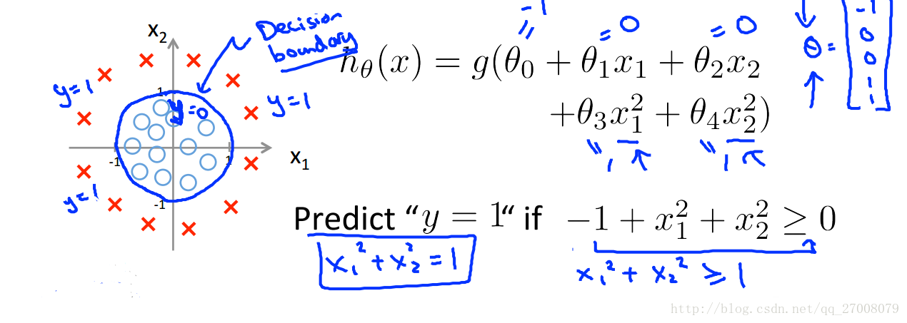
1.3 Decision boundary
-
y=1 if hθ(x)≥0.5,θTx≥0 -
y=0 if hθ(x)≤0.5,θTx≤0
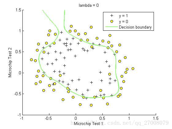
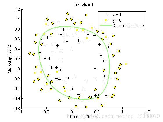
下面是两张图可以用来体会一下边界的含义
2.1 Cost function
让我们先来看看线性回归中的代价函数
假如我们将此函数用到逻辑回归中,会有什么问题呢?
因为假设函数
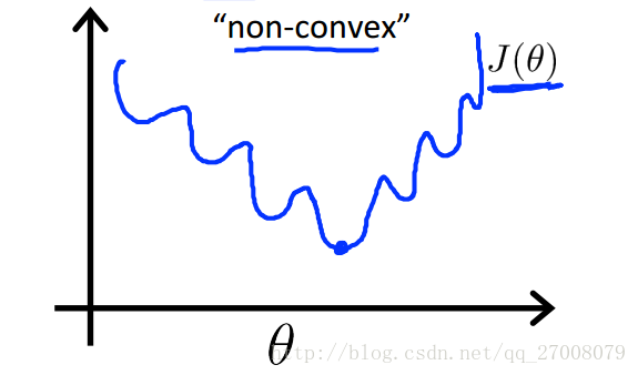
图像呈现出非凸性,也就是说,如果我们运用梯度下降法,不能保证算法收敛到全局最小值。
对于此问题,我们定义的代价函数如下所示
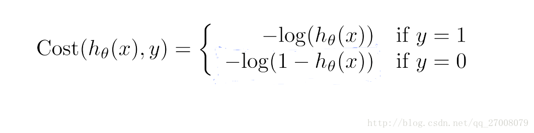
对上面的式子进行简化,总结如下。
Gradient Descent
Repeat{
}
算法看上去和线性回归保持一致
对于梯度下降法我们可以在matlab中使用如下高级函数
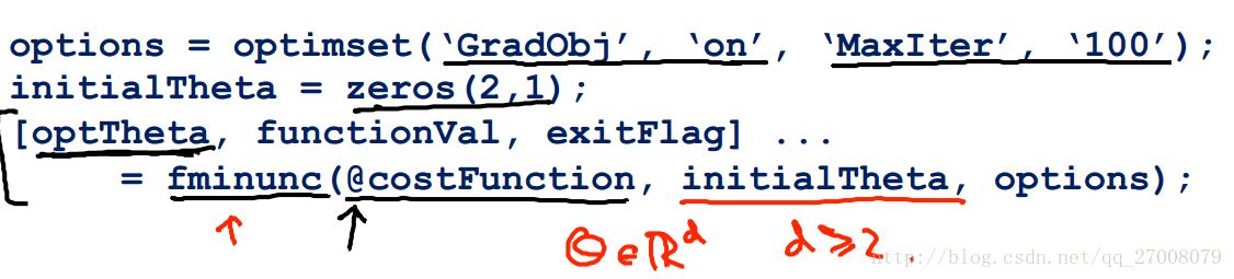
其中要定义代价函数costFunction:
2.2 Multiclass classification: One-vs-all
对于多分类,我们可以给每一类
来预测
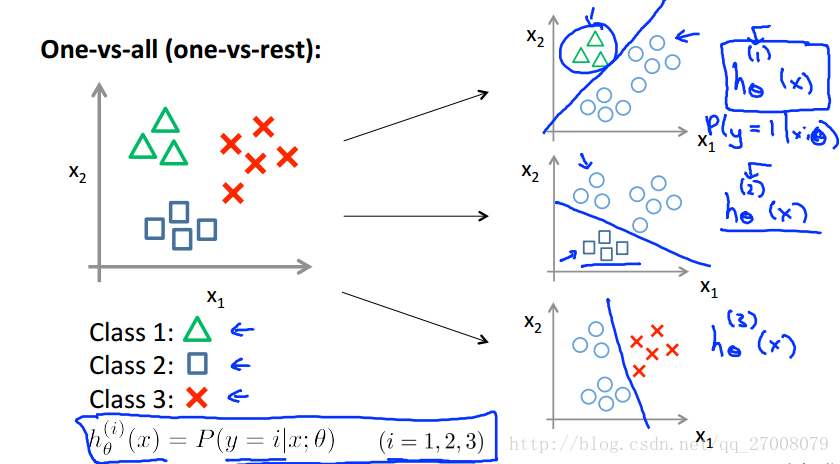
最终预测值为
3.1 The problem of overfitting
在数据拟合中,我们来看看下面三种情况。
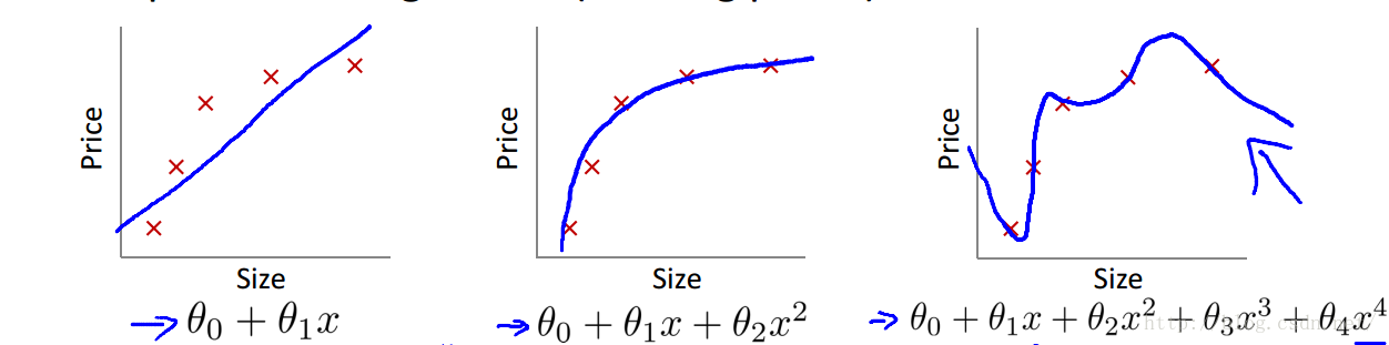
第一种称之为欠拟合,也叫高偏差,
第三种称之为过拟合,也叫高方差,在过拟合中,假设函数很好的匹配了训练集,但并不能很好的匹配测试集。
面对过拟合,我们有两种解决方式。
- 减少特征量。
- 含有所有特征量的情况下,减少
θj
3.2 Cost function
在采取第二种方式的情况下,我们应修改我们的代价函数如下
函数中,
这样一来修改下我们的梯度下降过程
Gradient Descent
Repeat{
}
逻辑回归时与以上情况类似。
作业代码
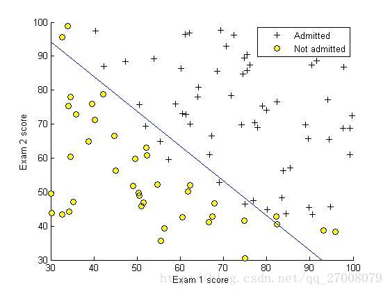
1.这次的作业任务是建立一个逻辑回归模型,判断一个学生能否被一个大学录取,给出的数据集为学生两门课的成绩和是否被录取,通过这些数据来预测一个学生能否被录取。
ex2.m
%% Machine Learning Online Class - Exercise 2: Logistic Regression
%
%  Instructions
%  ------------
%
%  This file contains code that helps you get started on the logistic
%  regression exercise. You will need to complete the following functions
%  in this exericse:
%
%     sigmoid.m
%     costFunction.m
%     predict.m
%     costFunctionReg.m
%
%  For this exercise, you will not need to change any code in this file,
%  or any other files other than those mentioned above.
%

%% Initialization
clear ; close all; clc

%% Load Data
%  The first two columns contains the exam scores and the third column
%  contains the label.

data = load('ex2data1.txt');
X = data(:, [1, 2]); y = data(:, 3);

%% ==================== Part 1: Plotting ====================
%  We start the exercise by first plotting the data to understand the
%  the problem we are working with.

fprintf(['Plotting data with + indicating (y = 1) examples and o ' ...
         'indicating (y = 0) examples.\n']);

plotData(X, y);

% Put some labels
hold on;
% Labels and Legend
xlabel('Exam 1 score')
ylabel('Exam 2 score')

% Specified in plot order
legend('Admitted', 'Not admitted')
hold off;

fprintf('\nProgram paused. Press enter to continue.\n');
pause;


%% ============ Part 2: Compute Cost and Gradient ============
%  In this part of the exercise, you will implement the cost and gradient
%  for logistic regression. You neeed to complete the code in
%  costFunction.m

%  Setup the data matrix appropriately, and add ones for the intercept term
[m, n] = size(X);

% Add intercept term to x and X_test
X = [ones(m, 1) X];

% Initialize fitting parameters
initial_theta = zeros(n + 1, 1);

% Compute and display initial cost and gradient
[cost, grad] = costFunction(initial_theta, X, y);

fprintf('Cost at initial theta (zeros): %f\n', cost);
fprintf('Expected cost (approx): 0.693\n');
fprintf('Gradient at initial theta (zeros): \n');
fprintf(' %f \n', grad);
fprintf('Expected gradients (approx):\n -0.1000\n -12.0092\n -11.2628\n');

% Compute and display cost and gradient with non-zero theta
test_theta = [-24; 0.2; 0.2];
[cost, grad] = costFunction(test_theta, X, y);

fprintf('\nCost at test theta: %f\n', cost);
fprintf('Expected cost (approx): 0.218\n');
fprintf('Gradient at test theta: \n');
fprintf(' %f \n', grad);
fprintf('Expected gradients (approx):\n 0.043\n 2.566\n 2.647\n');

fprintf('\nProgram paused. Press enter to continue.\n');
pause;


%% ============= Part 3: Optimizing using fminunc  =============
%  In this exercise, you will use a built-in function (fminunc) to find the
%  optimal parameters theta.

%  Set options for fminunc
options = optimset('GradObj', 'on', 'MaxIter', 400);

%  Run fminunc to obtain the optimal theta
%  This function will return theta and the cost
[theta, cost] = ...
    fminunc(@(t)(costFunction(t, X, y)), initial_theta, options);

% Print theta to screen
fprintf('Cost at theta found by fminunc: %f\n', cost);
fprintf('Expected cost (approx): 0.203\n');
fprintf('theta: \n');
fprintf(' %f \n', theta);
fprintf('Expected theta (approx):\n');
fprintf(' -25.161\n 0.206\n 0.201\n');

% Plot Boundary
plotDecisionBoundary(theta, X, y);

% Put some labels
hold on;
% Labels and Legend
xlabel('Exam 1 score')
ylabel('Exam 2 score')

% Specified in plot order
legend('Admitted', 'Not admitted')
hold off;

fprintf('\nProgram paused. Press enter to continue.\n');
pause;

%% ============== Part 4: Predict and Accuracies ==============
%  After learning the parameters, you'll like to use it to predict the outcomes
%  on unseen data. In this part, you will use the logistic regression model
%  to predict the probability that a student with score 45 on exam 1 and
%  score 85 on exam 2 will be admitted.
%
%  Furthermore, you will compute the training and test set accuracies of
%  our model.
%
%  Your task is to complete the code in predict.m

%  Predict probability for a student with score 45 on exam 1
%  and score 85 on exam 2

prob = sigmoid([1 45 85] * theta);
fprintf(['For a student with scores 45 and 85, we predict an admission ' ...
         'probability of %f\n'], prob);
fprintf('Expected value: 0.775 +/- 0.002\n\n');

% Compute accuracy on our training set
p = predict(theta, X);

fprintf('Train Accuracy: %f\n', mean(double(p == y)) * 100);
fprintf('Expected accuracy (approx): 89.0\n');
fprintf('\n');
sigmoid.m
function g = sigmoid(z)
%SIGMOID Compute sigmoid function
%   g = SIGMOID(z) computes the sigmoid of z.

% You need to return the following variables correctly
g = zeros(size(z));

% ====================== YOUR CODE HERE ======================
% Instructions: Compute the sigmoid of each value of z (z can be a matrix,
%               vector or scalar).

g = 1./(1 + exp(-z));

% =============================================================

end
costFunction.m
function [J, grad] = costFunction(theta, X, y)
%COSTFUNCTION Compute cost and gradient for logistic regression
%   J = COSTFUNCTION(theta, X, y) computes the cost of using theta as the
%   parameter for logistic regression and the gradient of the cost
%   w.r.t. to the parameters.

% Initialize some useful values
m = length(y); % number of training examples

% You need to return the following variables correctly
J = 0;
grad = zeros(size(theta));

% ====================== YOUR CODE HERE ======================
% Instructions: Compute the cost of a particular choice of theta.
%               You should set J to the cost.
%               Compute the partial derivatives and set grad to the partial
%               derivatives of the cost w.r.t. each parameter in theta
%
% Note: grad should have the same dimensions as theta
%
J = 1/m*(-y'*log(sigmoid(X*theta)) - (1-y)'*(log(1-sigmoid(X*theta))));
grad = 1/m * X'*(sigmoid(X*theta) - y);

% =============================================================

end
predict.m
function p = predict(theta, X)
%PREDICT Predict whether the label is 0 or 1 using learned logistic
%regression parameters theta
%   p = PREDICT(theta, X) computes the predictions for X using a
%   threshold at 0.5 (i.e., if sigmoid(theta'*x) >= 0.5, predict 1)

m = size(X, 1); % Number of training examples

% You need to return the following variables correctly
p = zeros(m, 1);

% ====================== YOUR CODE HERE ======================
% Instructions: Complete the following code to make predictions using
%               your learned logistic regression parameters.
%               You should set p to a vector of 0's and 1's
%
p = sigmoid(X * theta)>=0.5;

% =========================================================================
end
2.检测产品的质量的保证,根据训练集里每个产品经过两次检测和质量好坏,预测新产品经过两次检测后的接受与否。
ex2_reg.m
%% Machine Learning Online Class - Exercise 2: Logistic Regression
%
%  Instructions
%  ------------
%
%  This file contains code that helps you get started on the second part
%  of the exercise which covers regularization with logistic regression.
%
%  You will need to complete the following functions in this exericse:
%
%     sigmoid.m
%     costFunction.m
%     predict.m
%     costFunctionReg.m
%
%  For this exercise, you will not need to change any code in this file,
%  or any other files other than those mentioned above.
%

%% Initialization
clear ; close all; clc

%% Load Data
%  The first two columns contains the X values and the third column
%  contains the label (y).

data = load('ex2data2.txt');
X = data(:, [1, 2]); y = data(:, 3);

plotData(X, y);

% Put some labels
hold on;

% Labels and Legend
xlabel('Microchip Test 1')
ylabel('Microchip Test 2')

% Specified in plot order
legend('y = 1', 'y = 0')
hold off;


%% =========== Part 1: Regularized Logistic Regression ============
%  In this part, you are given a dataset with data points that are not
%  linearly separable. However, you would still like to use logistic
%  regression to classify the data points.
%
%  To do so, you introduce more features to use -- in particular, you add
%  polynomial features to our data matrix (similar to polynomial
%  regression).
%

% Add Polynomial Features

% Note that mapFeature also adds a column of ones for us, so the intercept
% term is handled
X = mapFeature(X(:,1), X(:,2));

% Initialize fitting parameters
initial_theta = zeros(size(X, 2), 1);

% Set regularization parameter lambda to 1
lambda = 1;

% Compute and display initial cost and gradient for regularized logistic
% regression
[cost, grad] = costFunctionReg(initial_theta, X, y, lambda);

fprintf('Cost at initial theta (zeros): %f\n', cost);
fprintf('Expected cost (approx): 0.693\n');
fprintf('Gradient at initial theta (zeros) - first five values only:\n');
fprintf(' %f \n', grad(1:5));
fprintf('Expected gradients (approx) - first five values only:\n');
fprintf(' 0.0085\n 0.0188\n 0.0001\n 0.0503\n 0.0115\n');

fprintf('\nProgram paused. Press enter to continue.\n');
pause;

% Compute and display cost and gradient
% with all-ones theta and lambda = 10
test_theta = ones(size(X,2),1);
[cost, grad] = costFunctionReg(test_theta, X, y, 10);

fprintf('\nCost at test theta (with lambda = 10): %f\n', cost);
fprintf('Expected cost (approx): 3.16\n');
fprintf('Gradient at test theta - first five values only:\n');
fprintf(' %f \n', grad(1:5));
fprintf('Expected gradients (approx) - first five values only:\n');
fprintf(' 0.3460\n 0.1614\n 0.1948\n 0.2269\n 0.0922\n');

fprintf('\nProgram paused. Press enter to continue.\n');
pause;

%% ============= Part 2: Regularization and Accuracies =============
%  Optional Exercise:
%  In this part, you will get to try different values of lambda and
%  see how regularization affects the decision coundart
%
%  Try the following values of lambda (0, 1, 10, 100).
%
%  How does the decision boundary change when you vary lambda? How does
%  the training set accuracy vary?
%

% Initialize fitting parameters
initial_theta = zeros(size(X, 2), 1);

% Set regularization parameter lambda to 1 (you should vary this)
lambda = 0;

% Set Options
options = optimset('GradObj', 'on', 'MaxIter', 400);

% Optimize
[theta, J, exit_flag] = ...
    fminunc(@(t)(costFunctionReg(t, X, y, lambda)), initial_theta, options);

% Plot Boundary
plotDecisionBoundary(theta, X, y);
hold on;
title(sprintf('lambda = %g', lambda))

% Labels and Legend
xlabel('Microchip Test 1')
ylabel('Microchip Test 2')

legend('y = 1', 'y = 0', 'Decision boundary')
hold off;

% Compute accuracy on our training set
p = predict(theta, X);

fprintf('Train Accuracy: %f\n', mean(double(p == y)) * 100);
fprintf('Expected accuracy (with lambda = 1): 83.1 (approx)\n');

%------------------------------------------------------------------------------------
initial_theta = zeros(size(X, 2), 1);

% Set regularization parameter lambda to 1 (you should vary this)
lambda = 1;

% Set Options
options = optimset('GradObj', 'on', 'MaxIter', 400);

% Optimize
[theta, J, exit_flag] = ...
    fminunc(@(t)(costFunctionReg(t, X, y, lambda)), initial_theta, options);

% Plot Boundary
plotDecisionBoundary(theta, X, y);
hold on;
title(sprintf('lambda = %g', lambda))

% Labels and Legend
xlabel('Microchip Test 1')
ylabel('Microchip Test 2')

legend('y = 1', 'y = 0', 'Decision boundary')
hold off;

% Compute accuracy on our training set
p = predict(theta, X);

fprintf('Train Accuracy: %f\n', mean(double(p == y)) * 100);
fprintf('Expected accuracy (with lambda = 1): 83.1 (approx)\n');

%--------------------------------------------------------------------------------------
initial_theta = zeros(size(X, 2), 1);

% Set regularization parameter lambda to 1 (you should vary this)
lambda = 10;

% Set Options
options = optimset('GradObj', 'on', 'MaxIter', 400);

% Optimize
[theta, J, exit_flag] = ...
    fminunc(@(t)(costFunctionReg(t, X, y, lambda)), initial_theta, options);

% Plot Boundary
plotDecisionBoundary(theta, X, y);
hold on;
title(sprintf('lambda = %g', lambda))

% Labels and Legend
xlabel('Microchip Test 1')
ylabel('Microchip Test 2')

legend('y = 1', 'y = 0', 'Decision boundary')
hold off;

% Compute accuracy on our training set
p = predict(theta, X);

fprintf('Train Accuracy: %f\n', mean(double(p == y)) * 100);
fprintf('Expected accuracy (with lambda = 1): 83.1 (approx)\n');

%------------------------------------------------------------------------------
initial_theta = zeros(size(X, 2), 1);

% Set regularization parameter lambda to 1 (you should vary this)
lambda = 100;

% Set Options
options = optimset('GradObj', 'on', 'MaxIter', 400);

% Optimize
[theta, J, exit_flag] = ...
    fminunc(@(t)(costFunctionReg(t, X, y, lambda)), initial_theta, options);

% Plot Boundary
plotDecisionBoundary(theta, X, y);
hold on;
title(sprintf('lambda = %g', lambda))

% Labels and Legend
xlabel('Microchip Test 1')
ylabel('Microchip Test 2')

legend('y = 1', 'y = 0', 'Decision boundary')
hold off;

% Compute accuracy on our training set
p = predict(theta, X);

fprintf('Train Accuracy: %f\n', mean(double(p == y)) * 100);
fprintf('Expected accuracy (with lambda = 1): 83.1 (approx)\n');
costFunctionReg.m
function [J, grad] = costFunctionReg(theta, X, y, lambda)
%COSTFUNCTIONREG Compute cost and gradient for logistic regression with regularization
%   J = COSTFUNCTIONREG(theta, X, y, lambda) computes the cost of using
%   theta as the parameter for regularized logistic regression and the
%   gradient of the cost w.r.t. to the parameters.

% Initialize some useful values
m = length(y); % number of training examples

% You need to return the following variables correctly
J = 0;
grad = zeros(size(theta));

% ====================== YOUR CODE HERE ======================
% Instructions: Compute the cost of a particular choice of theta.
%               You should set J to the cost.
%               Compute the partial derivatives and set grad to the partial
%               derivatives of the cost w.r.t. each parameter in theta
J = 1/m * (-y' * log(sigmoid(X*theta)) - (1 - y') * log(1 - sigmoid(X * theta))) + lambda/2/m*sum(theta(2:end).^2);

grad(1,:) = 1/m * (X(:, 1)' * (sigmoid(X*theta) - y));
grad(2:size(theta), :) = 1/m * (X(:, 2:size(theta))' * (sigmoid(X*theta) - y))...
        + lambda/m*theta(2:size(theta), :);
% =============================================================

end