决策树:和k近邻算法一样,也是用来做分类用的。简单地说就是将一个未知分类的事务依次通过多个判断条件,根据符不符合条件来进行分类,递归下降,直至判断出确定类型。PS.偷一张书上邮件分类的图嘻嘻....

决策树特性(本菜鸡认为的重点):
优点:复杂度不高,易于理解,中间值缺失不敏感(就是缺几个值也问题不大)
缺点:可能过度匹配
使用范围:数值型、标称型。
1、知识补充——信息增益
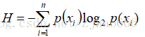
根据香农大佬钦定的基本法,符号xi的信息定义为

其中p(xi)是选择该分类的概率
信息期望值为
2、梳理实战代码
好了,有了信息熵的知识铺垫,我们可以开始了
首先创建trees.py文件
import operator
from math import log  # 通过math包导入log函数


# 计算给定数据的熵
def calcShannonEnt(dataSet):
    numEntries = len(dataSet)  # 数据集长度
    labelCounts = {}  # 定义标签字典
    for featVec in dataSet:
        currentLabel = featVec[-1]  # 最后一列数值,即标签数值
        if currentLabel not in labelCounts.keys():  # 若不存在
            labelCounts[currentLabel] = 0  # 添加入标签字典,并初始化为0
        labelCounts[currentLabel] += 1  # 标签频数自增
    shannonEnt = 0.0  # 定义香农熵,注意是浮点型,PS entropy 熵
    for key in labelCounts:  # 计算每个标签的香农熵
        prob = float(labelCounts[key]) / numEntries  # 计算频率
        shannonEnt -= prob * log(prob, 2)  # 代入之前的信息期望值公式
    return shannonEnt  # 返回香农熵


def createDataSet():
    # 数据集
    dataSet = [[1, 1, 'yes'],
               [1, 1, 'yes'],
               [1, 0, 'no'],
               [0, 1, 'no'],
               [0, 1, 'no']]
    # 标签集
    labels = ['no surfacing', 'flippers']
    return dataSet, labels
然后在命令行输入:
>>> from imp import reload
>>> import trees
>>> reload(trees)
<module 'trees' from 'C:\\Users\\dell\\PycharmProjects\\untitled\\trees.py'>
>>> myDat,labels=trees.createDataSet()
>>> myDat
[[1, 1, 'yes'], [1, 1, 'yes'], [1, 0, 'no'], [0, 1, 'no'], [0, 1, 'no']]
>>> trees.calcShannonEnt(myDat)
0.9709505944546686
结果正确,很开森!
决策树分类算法除了需要测量信息熵,还需要划分数据集,度量划分数据集的熵,以判断当前是否正确地划分了数据集。
好了,用正常人听得懂的话解释就是:在分类的过程中,将哪个属性作为新的判断结点,取决于这个属性是否为当前“最好的”分类标准。“最好”即用信息增益最大,即按照此种分类计算(之前的代码干的活)出的信息熵是最大的。
下面接着在trees.py中继续书写代码。
#参数解释
#dataSet 待划分的数据集
#axis 划分数据集的特征
#value 特征的返回值
def splitDataSet(dataSet, axis, value):
    # python的引用特性决定了不创建新的对象则在函数内部对列表对象的修改,将会影响该列表对象的整个生存周期
    retDataSet = []
    for featVec in dataSet:
        if featVec[axis] == value:#一旦在下标为axis的属性发现符合要求的值,即等于value,则将其添加到新创建的列表retDataSet中
            #python通过下标子序列中[a,b]实际上只取出下标为a到下标为b-1的所有元素
            #换句话说,featVec[:axis]就漏掉了featVec中下表为axis的元素
            reducedFeatVec = featVec[:axis]
            reducedFeatVec.extend(featVec[axis + 1:])#extend是将所有新元素直接加入序列中
            retDataSet.append(reducedFeatVec)#append是将所有新元素视作一个集合,然后再整体作为一个元素加入到序列中
    #返回决策树
    return retDataSet
接着,我们在命令行中输入:
>>> from imp import reload
>>> import trees
>>> reload(trees)
<module 'trees' from 'C:\\Users\\dell\\PycharmProjects\\untitled\\trees.py'>
>>> myDat,labels=trees.createDataSet()
>>> myDat
[[1, 1, 'yes'], [1, 1, 'yes'], [1, 0, 'no'], [0, 1, 'no'], [0, 1, 'no']]
>>> trees.splitDataSet(myDat,0,1)
[[1, 'yes'], [1, 'yes'], [0, 'no']]
>>> trees.splitDataSet(myDat,0,0)
[[1, 'no'], [1, 'no']]
下面,我们需要选择最好的数据集划分方式,即确定之前所说的分类结点
# 选择最好的数据集划分方式
# 选取特征,划分数据集,计算得出最好的划分数据集的特征
# dataSet要求:1、由列表组成的列表,而且所有的列表元素都要有相同的数据长度;2、数据的最后一列是实例的类别标签
def chooseBestFeatureToSplit(dataSet):
    numFeatures = len(dataSet[0]) - 1  # 取除了最后一个元素的前面其他所有属性
    baseEntropy = calcShannonEnt(dataSet)  # 香农熵
    bestInfoGain = 0.0  # 信息增益
    bestFeature = -1  # 最好分类标准的列表下标
    for i in range(numFeatures):
        # 通过set创建唯一的分类标签列表
        # 这种优秀列表创建方式可以学习一波
        # 特别注意,dataSet是由列表组成的列表,所以是example[i]而不是example,取出的实际上是一整个属性列
        featList = [example[i] for example in dataSet]
        uniqueVals = set(featList)  # 集合类属性唯一
        newEntropy = 0.0  # 浮点数注意
        # 计算每种划分方式的信息熵
        for value in uniqueVals:
            subDataSet = splitDataSet(dataSet, i, value)
            prob = len(subDataSet) / float(len(dataSet))
            newEntropy += prob * calcShannonEnt(subDataSet)
        infoGain = baseEntropy - newEntropy
        # 计算最好的信息增益
        if (infoGain > bestInfoGain):
            bestInfoGain = infoGain
            bestFeature = i
    #返回最优划分属性
    return bestFeature
接着在命令行中测试输入:
>>> reload(trees)
<module 'trees' from 'C:\\Users\\dell\\PycharmProjects\\untitled\\trees.py'>
>>> myDat,labels=trees.createDataSet()
>>> trees.chooseBestFeatureToSplit(myDat)
0
>>> myDat
[[1, 1, 'yes'], [1, 1, 'yes'], [1, 0, 'no'], [0, 1, 'no'], [0, 1, 'no']]
结果正确,开心!
加下来来学习构建递归构建决策树
首先定义函数majority,和之前k近邻算法中的classify0函数类似,不再赘述。
# classList 分类名称列表
# 可以参看之前k近邻算法中的classify0函数,就不再解释了
def majorityCnt(classList):
    classCount = {}
    for vote in classList:
        if vote not in classCount.keys(): classCount[vote] = 0;
        classCount[vote] += 1
    sortedClassCount = sorted(classCount.items(),
                              key=operator.itemgetter(1), reverse=True)
    return sortedClassCount[0][0]
接着正式递归构建决策树:
递归终止条件(满足其一即可):
(1)程序遍历完所有划分数据集的属性
(2)每个分支下的所有实例都具有相同的分类
接着输入代码
def createTree(dataSet, labels):
    # 最后一个是标签
    classList = [example[-1] for example in dataSet]
    # 类别完全相同则停止继续划分
    if classList.count(classList[0]) == len(classList):
        return classList[0]
    # 遍历玩所有特征时返回出现次数最多的
    if len(dataSet[0]) == 1:
        return majorityCnt(classList)
    bestFeat = chooseBestFeatureToSplit(dataSet)  # 找到最合适的分割
    bestFeatLabel = labels[bestFeat]
    myTree = {bestFeatLabel: {}}  # 开始构造决策树
    del (labels[bestFeat])  # 在原有标签中删除最佳分割属性
    featValues = [example[bestFeat] for example in dataSet]
    uniqueVals = set(featValues)  # 通过集合删除重复元素
    for value in uniqueVals:
        subLabels = labels[:]  # 拷贝剩下的标签数据
        myTree[bestFeatLabel][value] = createTree(splitDataSet(dataSet, bestFeat, value), subLabels)  # 此处用了递归的思想
    # 返回生成的生成树
    return myTree
在命令行中测试:
>>> from imp import reload
>>> import trees
>>> reload(trees)
<module 'trees' from 'C:\\Users\\dell\\PycharmProjects\\untitled\\trees.py'>
>>> myDat,labels=trees.createDataSet()
>>> myTree=trees.createTree(myDat,labels)
>>> myTree
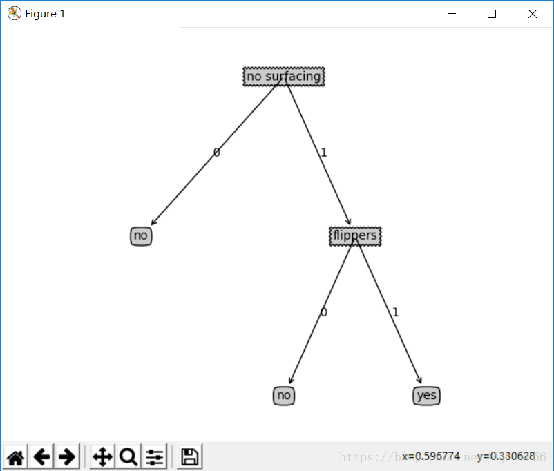
{'no surfacing': {0: 'no', 1: {'flippers': {0: 'no', 1: 'yes'}}}}
结果正确
接下来,我们来学习使用Matplotlib绘制树形图
创建treePlotter.py文件用于绘图,继续书写python代码 PS. plotter 绘图机
import matplotlib.pyplot as plt#引入matplotlib包中的pyplot

#判断结点
decisionNode = dict(boxstyle="sawtooth", fc="0.8")#boxstyle 文本框类型 sawtooth 锯齿形 fc 边框线粗细
#叶子节点
leafNode = dict(boxstyle="round4", fc="0.8")#round4 圆边
#箭头
arrow_args = dict(arrowstyle="<-")#arrowstyle 箭头风格
def plotNode(nodeTxt, centerPt, parentPt, nodeType):
    # annotate是关于一个数据点的文本
    # nodeTxt为要显示的文本,centerPt为文本的中心点,箭头所在的点,parentPt为指向文本的点
    createPlot.ax1.annotate(nodeTxt, xy=parentPt,  xycoords='axes fraction',\
             xytext=centerPt, textcoords='axes fraction',\
             va="center", ha="center", bbox=nodeType, arrowprops=arrow_args)
def createPlot():
   fig = plt.figure(1, facecolor='white')#背景为白色
   fig.clf()# 把画布清空
   # createPlot.ax1为全局变量,绘制图像的句柄,subplot为定义了一个绘图,111表示figure中的图有1行1列,即1个,最后的1代表第一个图
   createPlot.ax1 = plt.subplot(111, frameon=False)
   #绘制判断结点 名字 箭头 箭尾 结点类型
接着我们在命令行中测试我们的绘图代码
>>> import treePlotter
>>> treePlotter.createPlot()
绘图结果如下
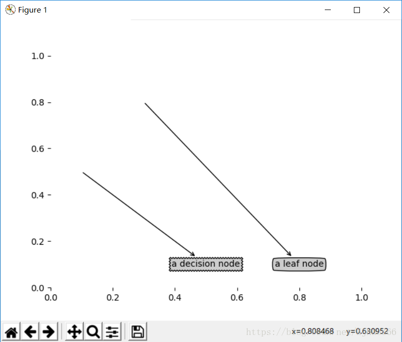
结果正确
接着,我们来构造注解树
首先我们要知道树有多少个叶子节点,以确定x轴的长度;还需要知道树有多少层,以确定y轴的高度。
在treePlotter.py中,定义getNumLeafs()获取叶子数目,定义getTreeDepth()获取树的层数,来,在treePlotter.py中接着敲代码如下:
#获取树的层数
def getTreeDepth(myTree):
    maxDepth = 0
    #python2 版本
    # firstStr = myTree.keys()[0]
    #python3 版本
    firstSides=list(myTree.keys())
    firstStr=firstSides[0]

    secondDict = myTree[firstStr]
    for key in secondDict.keys():
        if type(secondDict[key]).__name__ == 'dict':
            thisDepth = 1 + getTreeDepth(secondDict[key])
        else:#叶子节点在此处即条件为假,终止递归并直接返回,并将计算树深度的变量加一
            thisDepth = 1
        if thisDepth > maxDepth: maxDepth = thisDepth
    return maxDepth

#为节省时间,函数retrieveTrees输出预先存储的树信息,避免了每次测试代码时都要从数据中创建树的麻烦
#retrieve 取回,恢复
def retrieveTree(i):
    listOfTrees=[{'no surfacing':{0:'no',1:{'flippers':{0:'no',1:'yes'}}}},
                 {'no surfacing':{0:'no',1:{'flippers':{0:{'head':{0:'no',1:'yes'}},1:'no'}}}}
                 ]
    return listOfTrees[i]
接着在命令行中检测:
>>> reload(treePlotter)
<module 'treePlotter' from 'C:\\Users\\dell\\PycharmProjects\\untitled\\treePlotter.
py'>
>>> treePlotter.retrieveTree(1)
{'no surfacing': {0: 'no', 1: {'flippers': {0: {'head': {0: 'no', 1: 'yes'}}, 1: 'no
'}}}}
>>> myTree=treePlotter.retrieveTree(0)
>>> treePlotter.getNumLeafs(myTree)
3
>>> treePlotter.getTreeDepth(myTree)
2
现在,我们把之前的方法组合到一起,绘制一棵完整的树。现在继续完善treePlotter.py,并更新其中的createPlot()函数
在treePlotter中继续输入
# 在父子节点间填充文本信息
# 计算父节点和子节点的中间位置,并添加简单的文本标签信息
def plotMidText(cntrPt, parentPt, txtString):
    xMid = (parentPt[0] - cntrPt[0]) / 2.0 + cntrPt[0]
    yMid = (parentPt[1] - cntrPt[1]) / 2.0 + cntrPt[1]
    createPlot.ax1.text(xMid, yMid, txtString)  # 是ax1是一不是L


def plotTree(myTree, parentPt, nodeTxt):
    numLeafs = getNumLeafs(myTree)  # 宽
    depth = getTreeDepth(myTree)  # 高
    # python2版本
    # firstStr = myTree.keys()[0]
    # python3版本
    firstSides = list(myTree.keys())
    firstStr = firstSides[0]
    # totalW存储树的宽度
    # totalD存储树的深度
    cntrPt = (plotTree.xOff + (1.0 + float(numLeafs)) / 2.0 / plotTree.totalW, plotTree.yOff)
    # 标记子节点属性值
    # 计算父节点和子节点的中间位置,并添加简单的文本标签信息
    plotMidText(cntrPt, parentPt, nodeTxt)
    plotNode(firstStr, cntrPt, parentPt, decisionNode)
    secondDict = myTree[firstStr]
    # 减少y偏移
    # 按比例减少全局变量plotTree.yOff,并标注此处将要绘制子节点,既可以是叶子也可以是判断
    # 因为我们是自顶向下绘制图形,因此需要依次减少y坐标值,而不是递增y坐标值
    plotTree.yOff = plotTree.yOff - 1.0 / plotTree.totalD
    for key in secondDict.keys():
        if type(secondDict[key]).__name__ == 'dict':  # 不是叶子节点继续递归
            plotTree(secondDict[key], cntrPt, str(key))  # 递归遍历整棵树
        else:  # 是叶子节点画出叶子节点
            plotTree.xOff = plotTree.xOff + 1.0 / plotTree.totalW
            plotNode(secondDict[key], (plotTree.xOff, plotTree.yOff), cntrPt, leafNode)
            plotMidText((plotTree.xOff, plotTree.yOff), cntrPt, str(key))
    plotTree.yOff = plotTree.yOff + 1.0 / plotTree.totalD


# 创建绘图区,计算树形图全局尺寸,并递归调用函数plotTree()
def createPlot(inTree):
    fig = plt.figure(1, facecolor='white')  # 背景为白色
    fig.clf()  # 把画布清空
    axprops = dict(xticks=[], yticks=[])
    # createPlot.ax1为全局变量,绘制图像的句柄,subplot为定义了一个绘图,111表示figure中的图有1行1列,即1个,最后的1代表第一个图
    createPlot.ax1 = plt.subplot(111, frameon=False, **axprops)
    plotTree.totalW = float(getNumLeafs(inTree))
    plotTree.totalD = float(getTreeDepth(inTree))
    plotTree.xOff = -0.5 / plotTree.totalW;
    plotTree.yOff = 1.0;
    plotTree(inTree, (0.5, 1.0), '')
    # 展示图画
    plt.show()
命令行检测图形:
>>> reload(treePlotter)
<module 'treePlotter' from 'C:\\Users\\dell\\PycharmProjects\\untitled\\treePlotter.
py'>
>>> myTree=treePlotter.retrieveTree(0)
>>> treePlotter.createPlot(myTree)
图案如下:
接着,测试和存储分类器,把重心转移到如何利用决策树执行数据分类
将以下代码加入到trees.py中
def classify(inputTree, featLabels, testVec):
    firstSides = list(inputTree.keys())
    firstStr = firstSides[0]
    secondDict = inputTree[firstStr]
    # 查找当前列表中第一个匹配firstStr变量的元素
    featIndex = featLabels.index(firstStr)
    for key in secondDict.keys():
        if testVec[featIndex] == key:
            if type(secondDict[key]).__name__ == 'dict':
                #递归遍历整棵树
                classLabel = classify(secondDict[key], featLabels, testVec)
            else:
                classLabel = secondDict[key]
    return classLabel
下面接着套路般的命令行检测:
>>> reload(trees)
<module 'trees' from 'C:\\Users\\dell\\PycharmProjects\\untitled\\trees.py'>
>>> myDat,labels=trees.createDataSet()
>>> labels
['no surfacing', 'flippers']
>>> myTree=treePlotter.retrieveTree(0)
>>> myTree
{'no surfacing': {0: 'no', 1: {'flippers': {0: 'no', 1: 'yes'}}}}
>>> trees.classify(myTree,labels,[1,0])
'no'
>>> trees.classify(myTree,labels,[1,1])
'yes'
检测结果正确
感谢阅读到最后,发现错误欢迎指正。