版权声明:转载请注明出处 https://blog.csdn.net/GDFSG/article/details/53172192
这里把Sparse Autoencoder编程练习的代码和结果记录下来。
UFLDL源代码 http://ufldl.stanford.edu/wiki/index.php/Exercise:Sparse_Autoencoder
1. 部分代码
Sparse Autoencoder的练习需要完成sampleIMAGES.m、sparseAutoencoderCost.m、computeNumericalGradient.m三个程序文件。
主程序文件是train.m,先来看看train.m来对稀疏编码有个大致印象。
1.1 train.m(不需改动)
%% CS294A/CS294W Programming Assignment Starter Code%
%
%%======================================================================
%% STEP 0: 设置一些参数,这里不需要修改
visibleSize = 8*8;     % 输入节点个数
hiddenSize = 25;       % 输出节点个数
sparsityParam = 0.01;  % 隐层节点平均激活度,也就是教程里的稀疏性参数rho
lambda = 0.0001;       % 权重衰减参数
beta = 3;              % 稀疏权值惩罚项

%%======================================================================
%% STEP 1: 完成sampleIMAGES
%
%  采样完成后,display_newwork命令会显示其中的200个样本

patches = sampleIMAGES;
display_network(patches(:,randi(size(patches,2),200,1)),8);


%  参数随机初始化,theta是列向量(W1,W2,b1,b2)
theta = initializeParameters(hiddenSize, visibleSize);

%%======================================================================
%% STEP 2: 完成sparseAutoencoderCost
%
%  代价函数里需要计算平方误差代价、权值衰减项、稀疏惩罚三项。建议按以下步骤编写,
%  每写完一个进行一次梯度检验(step3)
%  (a) 先计算前向传播结果, 然后计算代价函数的平方误差项,再计算反向传播导数。
%      可以令lambda=beta=0,进行梯度检验确保平方误差代价计算正确
%  (b) 在代价函数和偏导中加入权重衰减项,进行梯度检验确保正确
%  (c) 添加稀疏惩罚项,进行梯度检验
%
%  运行成功后,可以尝试修改相关参数,如训练集大小、隐层节点数量、beta=lambda=0.

[cost, grad] = sparseAutoencoderCost(theta, visibleSize, hiddenSize, lambda, ...
                                     sparsityParam, beta, patches);

%%======================================================================
%% STEP 3: 梯度检验
%
% 本程序适用于小模型和小训练集。

% 先完成computeNumericalGradient.m,下面语句将检验程序是否正确
checkNumericalGradient();

% 计算代价和梯度
numgrad = computeNumericalGradient( @(x) sparseAutoencoderCost(x, visibleSize, ...
                                                  hiddenSize, lambda, ...
                                                  sparsityParam, beta, ...
                                                  patches), theta);

% 显示结果
disp([numgrad grad]);

% 比较数值计算得到的梯度和反向传播得到的梯度,正确的话相差应该小于1e-9
diff = norm(numgrad-grad)/norm(numgrad+grad);
disp(diff);

%%======================================================================
%% STEP 4: 使用L-BFGS对代价函数进行优化
%
%  随机初始化参数
theta = initializeParameters(hiddenSize, visibleSize);

%  使用minFunc进行优化
addpath minFunc/
options.Method = 'lbfgs'; % 这里使用L-BFGS优化代价函数,输出函数值和梯度
options.maxIter = 400;	  % L-BFGS最大迭代400次
options.display = 'on';


[opttheta, cost] = minFunc( @(p) sparseAutoencoderCost(p, ...
                                   visibleSize, hiddenSize, ...
                                   lambda, sparsityParam, ...
                                   beta, patches), ...
                              theta, options);

%%======================================================================
%% STEP 5: 可视化

W1 = reshape(opttheta(1:hiddenSize*visibleSize), hiddenSize, visibleSize);
display_network(W1', 12);

print -djpeg weights.jpg   % 保存成图片
我们需要完成step1、step2、step3的相关程序
1.2 sampleIMAGES.m
function patches = sampleIMAGES()
% 从训练集中采样10000个样本

load IMAGES;

patchsize = 8;  % 样本大小8×8
numpatches = 10000;

% 把patches初始化为0,这里patches尺寸是64×10000,每一列代表一个样本
patches = zeros(patchsize*patchsize, numpatches);

%% ---------- YOUR CODE HERE --------------------------------------
%  Instructions: Fill in the variable called "patches" using data
%  from IMAGES.
%
%  IMAGES is a 3D array containing 10 images
%  For instance, IMAGES(:,:,6) is a 512x512 array containing the 6th image,
%  and you can type "imagesc(IMAGES(:,:,6)), colormap gray;" to visualize
%  it. (The contrast on these images look a bit off because they have
%  been preprocessed using using "whitening."  See the lecture notes for
%  more details.) As a second example, IMAGES(21:30,21:30,1) is an image
%  patch corresponding to the pixels in the block (21,21) to (30,30) of
%  Image 1

[r,c,n]=size(IMAGES);
row = randi(r-patchsize+1,1,numpatches);
col = randi(c-patchsize+1,1,numpatches);
imgNum = randi(n,1,numpatches);
for i=1 : numpatches
   patch = IMAGES(row(i):row(i)+patchsize-1 , col(i):col(i)+patchsize-1 , imgNum(i));
   patches(:,i) = reshape(patch,patchsize*patchsize,1);
end

%% ---------------------------------------------------------------
% 把数据归一化到[0,1],因为后面要用到sigmoid激活函数
patches = normalizeData(patches);

end


%% ---------------------------------------------------------------
function patches = normalizeData(patches)
% 把数值归一化到[0,1]

% 去除DC成分 (图像均值).
patches = bsxfun(@minus, patches, mean(patches));
% 截尾为3倍的标准离差,调整为 -1 到 1
pstd = 3 * std(patches(:));
patches = max(min(patches, pstd), -pstd) / pstd;
% 从 [-1,1] 再调整为 [0.1,0.9]
patches = (patches + 1) * 0.4 + 0.1;

end
1.3 sparseAutocoderCost.m
function [cost,grad] = sparseAutoencoderCost(theta, visibleSize, hiddenSize, ...
                                             lambda, sparsityParam, beta, data)

% visibleSize: 输入节点数(这里是64)
% hiddenSize: 隐层节点数(这里是25)
% lambda: 权重衰减系数λ
% sparsityParam: 系数参数,隐层节点的平均激活度
% beta: 权重稀疏惩罚,train.m中设为常量
% data: 训练集,这里是64×10000的矩阵,data(:,i)表示第i个训练样本
%
% 根据initializeParameters.m所述,theta是把W和b随机初始化的结果,是一个列向量
% theta = [W1(:) ; W2(:) ; b1(:) ; b2(:)];

W1 = reshape(theta(1:hiddenSize*visibleSize), hiddenSize, visibleSize);
W2 = reshape(theta(hiddenSize*visibleSize+1:2*hiddenSize*visibleSize), visibleSize, hiddenSize);
b1 = theta(2*hiddenSize*visibleSize+1:2*hiddenSize*visibleSize+hiddenSize);
b2 = theta(2*hiddenSize*visibleSize+hiddenSize+1:end);
%注意W1是25×64的,W2是64×25的,b1是25×1的,b2是64×1的

% 代价和梯度值初始化
cost = 0;
W1grad = zeros(size(W1));
W2grad = zeros(size(W2));
b1grad = zeros(size(b1));
b2grad = zeros(size(b2));
%W1grad,即△W1;b1grad,即△b1

%% ---------- YOUR CODE HERE --------------------------------------
%  Instructions: Compute the cost/optimization objective J_sparse(W,b) for the Sparse Autoencoder,
%                and the corresponding gradients W1grad, W2grad, b1grad, b2grad.
%
% W1grad, W2grad, b1grad and b2grad should be computed using backpropagation.
% Note that W1grad has the same dimensions as W1, b1grad has the same dimensions
% as b1, etc.  Your code should set W1grad to be the partial derivative of J_sparse(W,b) with
% respect to W1.  I.e., W1grad(i,j) should be the partial derivative of J_sparse(W,b)
% with respect to the input parameter W1(i,j).  Thus, W1grad should be equal to the term
% [(1/m) \Delta W^{(1)} + \lambda W^{(1)}] in the last block of pseudo-code in Section 2.2
% of the lecture notes (and similarly for W2grad, b1grad, b2grad).
%
% Stated differently, if we were using batch gradient descent to optimize the parameters,
% the gradient descent update to W1 would be W1 := W1 - alpha * W1grad, and similarly for W2, b1, b2.
%
%%%%%%%%%%%%%%%%%%%%%%%%%%%%%%%%%%%%%%%%%%%%%%%%%%%%%%%%%%%%%
% Feedforward propagation
m = size(data,2);
z2 = W1*data+repmat(b1,1,m);   % = hiddenSize × m = 25 × 10000
a2 = sigmoid(z2);
z3 = W2*a2+repmat(b2,1,m);     % = visibleSize × m = 64 × 10000
a3 = sigmoid(z3);

% Cost function
% squared-error cost
cost1 = 1/2/m*sum(sum((a3-data).^2));
% weight decay cost
cost2 = lambda/2*(sum(sum(W1.^2))+sum(sum(W2.^2)));
% sparse constrain cost
rho0 = sparsityParam;
rho =  mean(a2,2);
kl = sum(rho0*log(rho0./rho) + (1-rho0)*log((1-rho0)./(1-rho)));
cost3 = beta*kl;
%total cost
cost = cost1 + cost2 + cost3;

% Error term
delta3 = -(data - a3).*a3.*(1-a3);
% delta2 need to add sparse penalty
KLgrad = beta * (-rho0 ./ rho + (1-rho0) ./ (1-rho)); % 25 x 1
KLgrad = repmat(KLgrad, 1, m);  % match the size of all examples
delta2 = (W2'*delta3+KLgrad).*a2.*(1-a2);

% Gradient
W1grad = delta2*data'/m + lambda*W1;
W2grad = delta3*a2'/m + lambda*W2;
b1grad = mean(delta2,2);
b2grad = mean(delta3,2);


%-------------------------------------------------------------------
% 计算完梯度,写成列向量形式,以便调用minFunc进行优化
grad = [W1grad(:) ; W2grad(:) ; b1grad(:) ; b2grad(:)];

end

%-------------------------------------------------------------------
% 定义sigmoid函数
function sigm = sigmoid(x)

    sigm = 1 ./ (1 + exp(-x));
end
1.4 computeNumericalGradient.m
function numgrad = computeNumericalGradient(J, theta)
% numgrad = computeNumericalGradient(J, theta)
% theta: 参数向量
% J: 调用y = J(theta)返回theta处的函数值

% 初始化numgrad
numgrad = zeros(size(theta));

%% ---------- YOUR CODE HERE --------------------------------------
% Instructions:
% Implement numerical gradient checking, and return the result in numgrad.
% (See Section 2.3 of the lecture notes.)
% You should write code so that numgrad(i) is (the numerical approximation to) the
% partial derivative of J with respect to the i-th input argument, evaluated at theta.
% I.e., numgrad(i) should be the (approximately) the partial derivative of J with
% respect to theta(i).
%
% Hint: You will probably want to compute the elements of numgrad one at a time.


EPSILON = 1e-4;
e = zeros(size(theta));
for i = 1:size(theta,1)
    e(i) = EPSILON;
    J1 = J(theta - e);
    J2 = J(theta + e);
    numgrad(i) = (J2 - J1) / (2*EPSILON);
    e(i) = 0;
end

%% ---------------------------------------------------------------
end
2. 结果
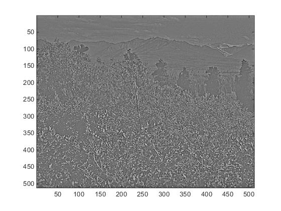
原始图片
运行 imagesc(IMAGES(:,:,6)), colormap gray;
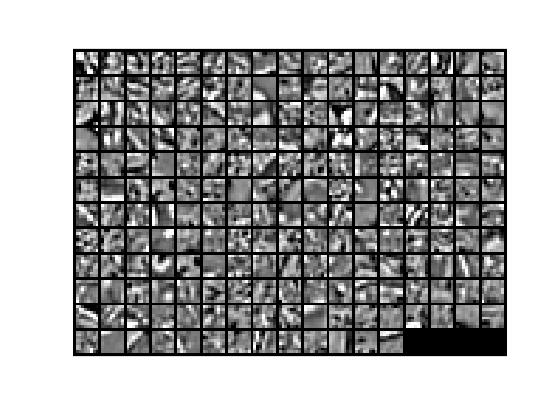
200个采样结果
运行 display_network(patches(:,randi(size(patches,2),200,1)),8);
最终输出结果
运行 print -djpeg weights.jpg
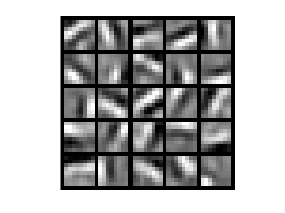
和教程里的正确答案类似,是一些边缘图像