在学习《深度学习》时,我主要是通过Andrew Ng教授在http://deeplearning.stanford.edu/wiki/index.php/UFLDL_Tutorial上提供的UFLDL(Unsupervised Feature Learning and Deep Learning)教程,本文在写的过程中,多有借鉴这个网站提供的资料。
稀疏自编码器(Sparse Autoencoder)可以自动从无标注数据中学习特征,可以给出比原始数据更好的特征描述。在实际运用时可以用稀疏编码器发现的特征取代原始数据,这样往往能带来更好的结果。本文将给出稀疏自编码器的算法描述,并演示说明稀疏编码器自动提取边缘特征。
转载请注明出处:http://blog.csdn.net/u010278305。
稀疏自编码器是具有一层隐含层的神经网络,其思路是让输出等于输入,(即 ,其中
,其中 表示训练样本集合),让编码器自己发现输入数据中隐含的特征,自编码神经网咯的结果如下图:

 的函数。换句话说,它尝试逼近一个恒等函数,从而使得输出
  接近于输入
接近于输入  。这样往往可以发现输入数据的一些有趣特征,最终我们会用隐藏层的神经元代替原始数据。当隐藏神经元数目少于输入的数目时,自编码神经网络可以达到数据压缩的效果(因为最终我们可以用隐藏神经元替代原始输入,输入层的n个输入转换为隐藏层的m个神经元,其中n>m,之后隐藏层的m个神经元又转换为输出层的n个输出,其输出等于输入);当隐藏神经元数目较多时,我们仍然可以对隐藏层的神经元加入稀疏性限制来发现输入数据的有趣结构。
稀疏性可以被简单地解释如下。如果当神经元的输出接近于1的时候我们认为它被激活,而输出接近于0的时候认为它被抑制,那么使得神经元大部分的时间都是被抑制的限制则被称作稀疏性限制。这里我们假设的神经元的激活函数是sigmoid函数(如果你使用tanh作为激活函数的话,当神经元输出为-1的时候,我们认为神经元是被抑制的)。
我们使用  来表示在给定输入为 情况下,自编码神经网络隐藏神经元
  的激活度。并将隐藏神经元 的平均活跃度(在训练集上取平均)记为:
![\begin{align}\hat\rho_j = \frac{1}{m} \sum_{i=1}^m \left[ a^{(2)}_j(x^{(i)}) \right]\end{align}](http://deeplearning.stanford.edu/wiki/images/math/8/7/2/8728009d101b17918c7ef40a6b1d34bb.png)
 其中
其中
 是稀疏性参数,
通常是一个接近于0的较小的值(比如
是稀疏性参数,
通常是一个接近于0的较小的值(比如
 ),换句话说,我们想要让隐藏神经元
的平均活跃度接近0.05。为了满足这一条件,隐藏神经元的活跃度必须接近于0。为了实现这一限制,我们需要在原始的神经网络优化目标函数中加入稀疏性限制这一项,作为一项额外的惩罚因子,我们可以选择具有如下形式的惩罚因子:
),换句话说,我们想要让隐藏神经元
的平均活跃度接近0.05。为了满足这一条件,隐藏神经元的活跃度必须接近于0。为了实现这一限制,我们需要在原始的神经网络优化目标函数中加入稀疏性限制这一项,作为一项额外的惩罚因子,我们可以选择具有如下形式的惩罚因子:
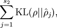
 是隐藏层中隐藏神经元的数量,而索引
依次代表隐藏层中的每一个神经元。该表达式也可以描述为
相对熵,记为
是隐藏层中隐藏神经元的数量,而索引
依次代表隐藏层中的每一个神经元。该表达式也可以描述为
相对熵,记为
-
-
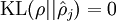
其中,
 是一个以
为均值和一个以
是一个以
为均值和一个以
 为均值的两个伯努利随机变量之间的相对熵。相对熵是一种标准的用来测量两个分布之间差异的方法。
-
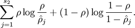
这一惩罚因子有如下性质,当
 时 ,
时 ,
 ,并且随着
与
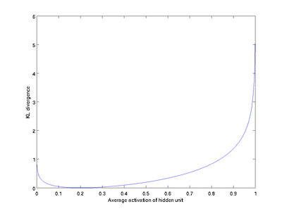
之间的差异增大而单调递增。举例来说,在下图中,我们设定
,并且随着
与
之间的差异增大而单调递增。举例来说,在下图中,我们设定
 并且画出了相对熵值
 随着
变化的变化。
随着
变化的变化。
-
-
我们可以看出,相对熵在
时达到它的最小值0,而当
靠近0或者1的时候,相对熵则变得非常大(其实是趋向于
 )。所以,最小化这一惩罚因子具有使得
靠近
的效果。现在,我们的总体代价函数可以表示为
)。所以,最小化这一惩罚因子具有使得
靠近
的效果。现在,我们的总体代价函数可以表示为

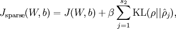
其中,  如之前所定义,而
  控制稀疏性惩罚因子的权重。 项则也(间接地)取决于
  ,因为它是隐藏神经元 的平均激活度,而隐藏层神经元的激活度取决于 。为此,我们需要相应更改第二层的导数,具体来说,就是将原来的导数
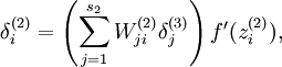
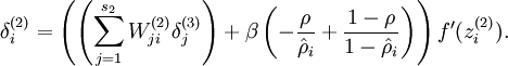
就可以了。
更新这个导数时,我们需要知道 这一项,因此在计算神经元的后向传播之前,需要对所有的训练样本计算一遍前向传播,从而获得平均激活度。
按照 http://deeplearning.stanford.edu/wiki/index.php/Exercise:Sparse_Autoencoder 给出的教程,我们可以对稀疏自编码器进行编写实现。
下面,给出稀疏自编码器代价函数及其导数的matlab代码实现:
function [cost,grad] = sparseAutoencoderCost(theta, visibleSize, hiddenSize, ...
                                             lambda, sparsityParam, beta, data)

% visibleSize: the number of input units (probably 64)
% hiddenSize: the number of hidden units (probably 25)
% lambda: weight decay parameter
% sparsityParam: The desired average activation for the hidden units (denoted in the lecture
%                           notes by the greek alphabet rho, which looks like a lower-case "p").
% beta: weight of sparsity penalty term
% data: Our 64x10000 matrix containing the training data.  So, data(:,i) is the i-th training example.

% The input theta is a vector (because minFunc expects the parameters to be a vector).
% We first convert theta to the (W1, W2, b1, b2) matrix/vector format, so that this
% follows the notation convention of the lecture notes.

W1 = reshape(theta(1:hiddenSize*visibleSize), hiddenSize, visibleSize);
W2 = reshape(theta(hiddenSize*visibleSize+1:2*hiddenSize*visibleSize), visibleSize, hiddenSize);
b1 = theta(2*hiddenSize*visibleSize+1:2*hiddenSize*visibleSize+hiddenSize);
b2 = theta(2*hiddenSize*visibleSize+hiddenSize+1:end);

% Cost and gradient variables (your code needs to compute these values).
% Here, we initialize them to zeros.
cost = 0;
W1grad = zeros(size(W1));
W2grad = zeros(size(W2));
b1grad = zeros(size(b1));
b2grad = zeros(size(b2));

%% ---------- YOUR CODE HERE --------------------------------------
%  Instructions: Compute the cost/optimization objective J_sparse(W,b) for the Sparse Autoencoder,
%                and the corresponding gradients W1grad, W2grad, b1grad, b2grad.
%
% W1grad, W2grad, b1grad and b2grad should be computed using backpropagation.
% Note that W1grad has the same dimensions as W1, b1grad has the same dimensions
% as b1, etc.  Your code should set W1grad to be the partial derivative of J_sparse(W,b) with
% respect to W1.  I.e., W1grad(i,j) should be the partial derivative of J_sparse(W,b)
% with respect to the input parameter W1(i,j).  Thus, W1grad should be equal to the term
% [(1/m) \Delta W^{(1)} + \lambda W^{(1)}] in the last block of pseudo-code in Section 2.2
% of the lecture notes (and similarly for W2grad, b1grad, b2grad).
%
% Stated differently, if we were using batch gradient descent to optimize the parameters,
% the gradient descent update to W1 would be W1 := W1 - alpha * W1grad, and similarly for W2, b1, b2.
%
m=size(data,2);

x=data;
a1=x;
z2=W1*a1+repmat(b1,1,m);
a2=sigmoid(z2);
z3=W2*a2+repmat(b2,1,m);
a3=sigmoid(z3);
h=a3;
y=x;
squared_error=0.5*sum((h-y).^2,1);
rho=1/m*sum(a2,2);
sparsity_penalty= beta*sum(sparsityParam.*log(sparsityParam./rho)+(1-sparsityParam).*log((1-sparsityParam)./(1-rho)));
cost=1/m*sum(squared_error)+lambda/2*(sum(sum(W1.^2))+sum(sum(W2.^2))) + sparsity_penalty;


grad_z3=a3.*(1-a3);
delta_3=-(y-a3).*grad_z3;
grad_z2=a2.*(1-a2);
delta_2=(W2'*delta_3+repmat(beta*(-sparsityParam./rho+(1-sparsityParam)./(1-rho)),1,m)).*grad_z2;
Delta_W2=delta_3*a2';
Delta_b2=sum(delta_3,2);
Delta_W1=delta_2*a1';
Delta_b1=sum(delta_2,2);
W1grad=1/m*Delta_W1+lambda*W1;
W2grad=1/m*Delta_W2+lambda*W2;
b1grad=1/m*Delta_b1;
b2grad=1/m*Delta_b2;


%-------------------------------------------------------------------
% After computing the cost and gradient, we will convert the gradients back
% to a vector format (suitable for minFunc).  Specifically, we will unroll
% your gradient matrices into a vector.

grad = [W1grad(:) ; W2grad(:) ; b1grad(:) ; b2grad(:)];

end

%-------------------------------------------------------------------
% Here's an implementation of the sigmoid function, which you may find useful
% in your computation of the costs and the gradients.  This inputs a (row or
% column) vector (say (z1, z2, z3)) and returns (f(z1), f(z2), f(z3)).

function sigm = sigmoid(x)

    sigm = 1 ./ (1 + exp(-x));
end
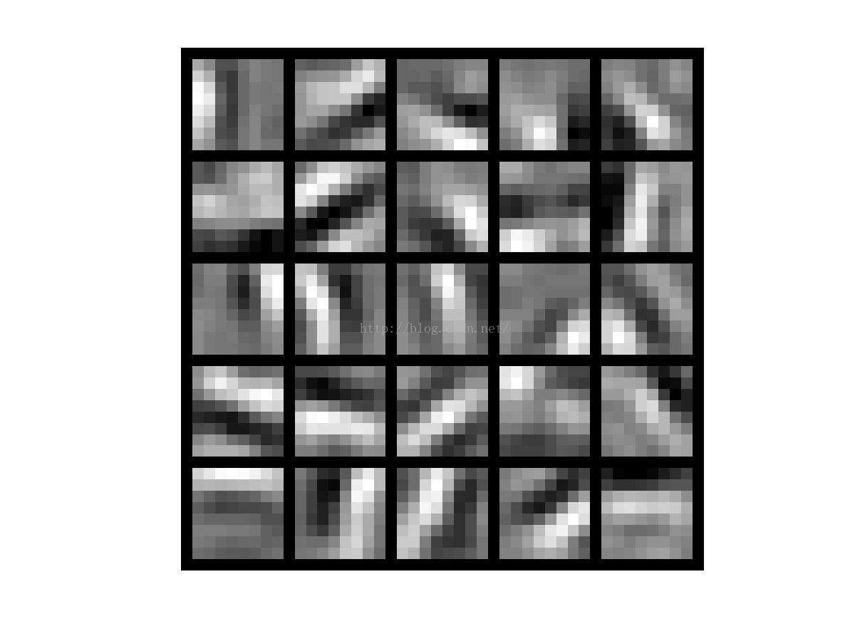
可以发现,稀疏自编码器可以自动提取输入图片的边缘特征。
稀疏自编码器完整的MATLAB实现代码已经上传,地址http://download.csdn.net/detail/u010278305/8901005
转载请注明出处:http://blog.csdn.net/u010278305