PCA主成分分析---降维（python调用实现）

使用鸢尾花数据集，原始特征向量为4，现在使用python库 降维为2维

import matplotlib.pyplot as plt  # 加载matplotlib用于数据的可视化
from sklearn.decomposition import PCA  # 加载PCA算法包
from sklearn.datasets import load_iris

data = load_iris()
y = data.target
x = data.data
pca = PCA(n_components=2)  # 加载PCA算法，设置降维后主成分数目为2
reduced_x = pca.fit_transform(x)  # 对样本进行降维
print(pca.components_) # 输出主成分，即行数为降维后的维数，列数为原始特征向量转换为新特征的系数
print(pca.explained_variance_) # 新特征 每维所能解释的方差大小
print(pca.explained_variance_ratio_) #新特征 每维所能解释的方差大小在全方差中所占比例

red_x, red_y = [], []
blue_x, blue_y = [], []
green_x, green_y = [], []

for i in range(len(reduced_x)):
    if y[i] == 0:
        red_x.append(reduced_x[i][0])
        red_y.append(reduced_x[i][1])
    elif y[i] == 1:
        blue_x.append(reduced_x[i][0])
        blue_y.append(reduced_x[i][1])
    else:
        green_x.append(reduced_x[i][0])
        green_y.append(reduced_x[i][1])
# 可视化
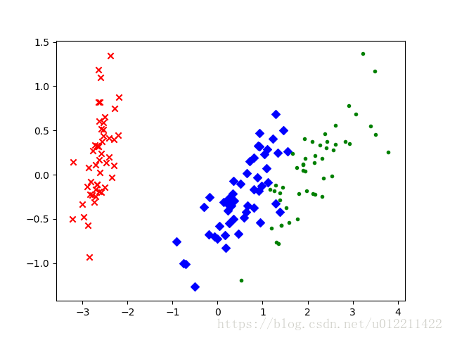
plt.scatter(red_x, red_y, c='r', marker='x')
plt.scatter(blue_x, blue_y, c='b', marker='D')
plt.scatter(green_x, green_y, c='g', marker='.')
plt.show()

运行结果：

[[ 0.36158968 -0.08226889  0.85657211  0.35884393]
 [ 0.65653988  0.72971237 -0.1757674  -0.07470647]]
[4.22484077 0.24224357]
[0.92461621 0.05301557]

参考链接：

[1]http://scikit-learn.org/stable/modules/generated/sklearn.decomposition.PCA.html

[2]https://blog.csdn.net/i_is_a_energy_man/article/details/76599400