非线性回归：逻辑回归（ Logistic Regression ）笔记

Logistic Regression (逻辑回归)

1. 基本模型

测试数据为X（x0，x1，x2···xn）

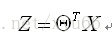
要学习的参数为： Θ（θ0，θ1，θ2，···θn）

向量表示：

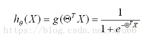
处理二值数据，引入Sigmoid函数时曲线平滑化：

得到逻辑回归的预测函数：

也可以用概率表示：

正例(y=1)，即在给定的x和Θ的情况下，发生的概率为：

反例(y=0)，即在给定的x和Θ的情况下，发生的概率为：

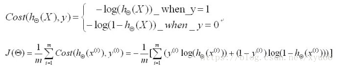
2 .cost函数

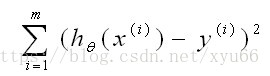
在线性回归中，预测值和真实值的差的平方，使其最小化。

在逻辑回归中，方程的合并过程，去对数有助于简化和易于判断单调性：

找到一组Θ值使以上方程最小化，利用梯度下降法。

梯度下降法：

按一定的学习率和更新法则，不断循环求导

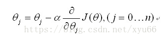
为找到最小值，对求偏导化简得到，逻辑回归的更新法则变为：

同时对所有的θ进行更新，重复更新直到收敛

3. python举例：

import numpy as np
import random


def gradientDescent(x, y, theta, alpha, m, numIterations):   # 梯度下降算法,x:实例, y:列, theta:θ, alpha:学习率,
                                                             # m:实例个数,numIterations:更新法则的次数
    xTrans = x.transpose()          # 转置矩阵
    for i in range(0, numIterations):   # numIterations=1000的话，循环从0到999
        hypothesis = np.dot(x, theta)   # hypothesis 内积 x和theta点乘
        loss = hypothesis - y           # hypothesis表示预测出来的y值

        cost = np.sum(loss ** 2) / (2 * m)

        print("Iteration %d | Cost: %f" % (i, cost))

        grandient = np.dot(xTrans, loss) / m

        theta = theta - alpha * grandient
    return theta


def getData(numPoints, bias, variance):    # 创建数据，参数为实例个数，偏好，方差
    x = np.zeros(shape=(numPoints, 2))     # numpoints行，2列
    y = np.zeros(shape=numPoints)           #label 标签

    for i in range(0, numPoints):      # 循环赋值，0到numpoints-1

        x[i][0] = 1
        x[i][1] = i

        y[i] = (i + bias) + random.uniform(0, 1) * variance      # uniform是从0到1之间随机取
    return x, y


x, y = getData(100, 25, 10)     # 100行即100个实例

# print("x:\n", x)
# print("y:\n", y)

m, n = np.shape(x)
# y_col = np.shape(y)

# print("x shape:", str(m), str(n))
# print("y shape:", str(y_col))

numIterations = 100000
alpha = 0.0005
theta = np.ones(n)      # 初始化为1
theta = gradientDescent(x, y, theta, alpha, m, numIterations)   # m=100个实例
print(theta)

θ更新，重复更新直到收敛，得到[29.68959795 1.01793798]

当有新的输入，带入可得到预测结果。

非线性回归：逻辑回归（ Logistic Regression ）笔记

猜你喜欢