Reinforcement Learning(强化学习)Sarsa/Q_learning

在说这两种算法之前，先说一下：

蒙特卡罗的方法（MC）和动态规划的方法（DP）

蒙特卡罗方法利用经验平均估计状态的值函数即：

这里的是状态后直到终止状态所有回报的返回值，也就是要得到实验结束才可以进行更新，这样的话太慢。

动态规划说的是可以用后继状态的值函数来估计当前的值函数即

这里的和如果有模型的话就可以根据当前的通过一个策略（这个策略在强化学习中一般就是选取具有最大奖励值的行动）确定下一步的行为a进而得到即：

所以两者结合一下就是时间差分学习TD,即改变一下，

这里其实就是将用了动态规划

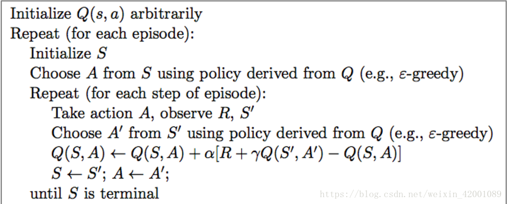
Sarsa即为：

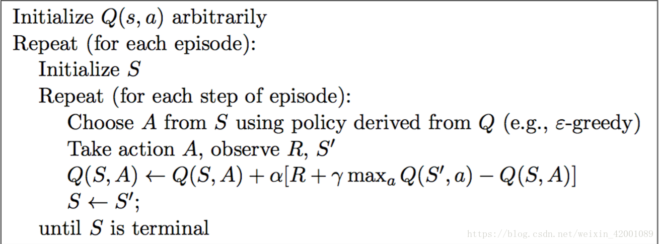
Q_learning即为：

所以Q_learning的特别就在于红色，动作值函数更新则不同于选取动作时遵循的策略,也就是说更新Q值的时候，直接使用了中最大的值——并且与当前执行的策略，即选取动作时采用的策略无关。

更多MC/DP/TD比较见https://zhuanlan.zhihu.com/p/25913410中讨论。

下面是详细分析：

Sarsa和Q_learning的算法核心分别是：

下面的分析用S代表状态，a代表S状态下采取的下一步行动，代表状态S下采取a行动后达到的状态，R代表状态S下采取a行动后的当前奖励值，

即Q表=  

	a0	a1	..............	am
S0
S1
S2
..........
Sn

选择下一步的行动A时的选择策略policy时两者没有什么不同，例如在考虑greedy的前提下，选取该状态下最大的A值即可（就是该S下这一行中最大的值）

Sarsa的步骤是:

                          （1） 根据初始化环境后得到初始状态S

                          （2）根据S通过policy选取下一步的行动a

                          （3）执行动作a，得到新的状态和R以及结束标志

                          （4）根据通过policy选取下一步的行动

                          （5）更新Q表：

                          （6）令S=  a=

                            ( 7)   判断结束标志是否是真，如果是，则结束，否则从第三步再次开始

Q_learning的步骤是：

                          （1） 根据初始化环境后得到初始状态S

                          （2）根据S通过policy选取下一步的行动a

                          （3）执行动作a，得到新的状态和R以及结束标志

                          （4）更新Q表：

                          （5）令S= 

                            ( 6)   判断是否遇到结束标志，如果遇到，则结束，否则从第二步再次开始

分析：

红色部分正是两者的核心，也正是上面两幅图的给出的关键部分，两者最大不同就是Sarsa是真真采取了行动，然后用采取后的结果去更新Q表，而Q_learning是假想的说：下一步要采取当前状态S一行中最大值的那个行动a，以此来更新Q表，但是等到真要走下一步的时候，并不一定是采取最大值对应的那个行动a，因为选取策略的policy此时依据的 已经变了，（就是 那一行的值已经变了，因为Q表已经提前依据“ 下一步就走最大值 ”的理论更新变了）

再说的简单一点就是，通过观察两者的步骤，Sarsa无非就是多了一步

（4）根据通过policy选取下一步的行动

然后Sarsa就是以下一步去更新Q表，而Q_learning则是“一根筋”就是认为下一步就是应该选择做大值对应的行动a，以此更新Q表。

通过Sarsa的（6）-----》（3）可以看出Sarsa对应的算法是下一步确实走了，而通过Q_learning的（5）-----》（2）可以看出选出的下一步行动并不一定是最大值（此时依据的S已经变了【就是Q表已经变了】）

正是因为Sarsa每一次的Q表更新都是依据真实的下一步行动，所以也叫做在线学习（on-policy）,对应的Q_learning就是离线学习（Off-policy）,Q_learning一般来说比较心急，一心只想着成功，因为它每次在更新Q表时，只是一门心思的想着最大值对应的行动，除了我要快点成功之外别的啥也不考虑，而Sarsa则相对来说比较谨慎，它会考虑真实下一步执行所带来的后果，总的来说：   Q_learning大步向前，勇者无敌！！！ ！！      Sarsa谨小慎微，步步为营！！！！！！！

#################################################################################################

假如要玩n次回合

Sarsa的框架可以简单的概括为：

for episode in range(n):
    #(1)         
    S = environment.reset()
    #(2)
    a = Sarsa.policy(str(observation))
    while True:
            # 环境刷新
            environment.render()

            # (3)
            S', R, Flage = environment.step(a)

            # (4)
            a' = Sarsa.policy(S')

            # (5)
            Sarsa.learn(S, a, R, S', a')

            # (6)
            S = S'
            a = a'
          
            # (7)
            if Flage:
                break

Q_learning的框架可以简单的概括为：   

for episode in range(n):
        
        # (1)
        S = environment.reset()
       

        while True:
            # 环境刷新
            environment.render()

            # (2)
            a= Q_learning.policy(S)

            # (3)
            S', R, Flage= environment.step(a)

            # (4)
            Q_learning.learn(S, a, R, S')

            # (5)
            S = S'

            # (6)
            if Flage:
                break

################################################################################################

正是由于Sarsa的谨小慎微，所以它会刻意的去避免奖励值少（或奖励值为负的惩罚）的行为，所以在 ”完成任务” 和 “躲避惩罚”

两者中其更看重后者，这就导致它有时候为了躲避而躲避，一直循环在一个局部，不敢出来，导致效率不高，针对这一问题有了改进版的Sarsa：

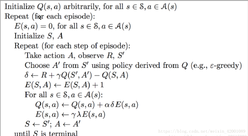
从中可以看到这里多了一个矩阵即,其维数和一样，每采取行动a后就给该矩阵对应的地方加一，然后又通过

进行衰减（因为和均小于1），其实这里相对于做标记，每经过某一步就给该步一个高度为1的脉冲，我们假设两种情况：

当结束标志为我们要的结果时（比如玩走迷宫游戏，此时对应的状态就是出口）那么上一步应该很重要，此时这个步骤也相应的得到了高度为1的脉冲，那么上上步呢？虽然其在上上步的过程中也得到了高度为1的脉冲但是其也经历了两次的衰减，上上上步，其在上上上步也得到了高度为1的脉冲，但其经历了三次衰减，所以距离我们目标越近的步骤其值越高，越远的步骤其值越小，尽管其也曾得到了脉冲，但经历了步步衰减，其值也很小了，然后又由于目前是我们想要的结果，奖励值会很高，即很高，所以此时再乘以 E(s,a)，那么就是相当于这一路探索下来的一系列行为中距离想要结果越近的行动值越高，越重要，依次来更新Q表，

当结束标志为一些惩罚时（比如玩走迷宫游戏，此时对应的状态就是障碍）那么此时会比较低（负数比较大），那么乘以 E(s,a)后导致的结果就是距离惩罚步骤的行动值高大（负数更大），危险系数更高。

除此之外每次加一，会导致一些重复的行为的值很高（没有上限嘛！），所以另一种方法就是说，将

改为：,也就是脉冲最高为1，可以想象到E矩阵中每一个状态对应的所有行动中，只有最后一次走过的那一个行为有值（>0）,其他值都是等于0的，也就是说最后的E矩阵中每一行中最多有一个值大于0，其它均为0.

下面来想一下其是如何解决单纯Sarsa所遇到的半天跳不出局部的问题的，一开始也就是玩第一局的话没有什么不同，但是随着局数增多，得到的q表应该是对于距离想要结果的有益的行为应该基于了更高的值，也就是距离目标越近的步骤值越高，所以Sarsa也会一心想着目标前进，而不是萎缩在一个循环里。

注意：Q_learning和单纯的Sarsa在更新Q表时是更新矩阵中对应的一个值。

        而改进的Sarsa更新的时候是用到整个矩阵的

这就是通俗的理解，想要更理论的理解，还需根据实际例子去看矩阵的变化，这里贴一下大神的莫凡的几个例子

地址：https://github.com/MorvanZhou/Reinforcement-learning-with-tensorflow

莫凡大神的demo分为三部分，一部分是游戏环境，一部分是强化学习的方法RL（就是Q_learning、Sarsa以及改进的Sarsa），另一部分就是run了

Q_learning：

环境：

"""
Reinforcement learning maze example.

Red rectangle:          explorer.
Black rectangles:       hells       [reward = -1].
Yellow bin circle:      paradise    [reward = +1].
All other states:       ground      [reward = 0].

This script is the environment part of this example. The RL is in RL_brain.py.

View more on my tutorial page: https://morvanzhou.github.io/tutorials/
"""


import numpy as np
import time
import sys
if sys.version_info.major == 2:
    import Tkinter as tk
else:
    import tkinter as tk


UNIT = 40   # pixels
MAZE_H = 4  # grid height
MAZE_W = 4  # grid width


class Maze(tk.Tk, object):
    def __init__(self):
        super(Maze, self).__init__()
        self.action_space = ['u', 'd', 'l', 'r']
        self.n_actions = len(self.action_space)
        self.title('maze')
        self.geometry('{0}x{1}'.format(MAZE_H * UNIT, MAZE_H * UNIT))
        self._build_maze()

    def _build_maze(self):
        self.canvas = tk.Canvas(self, bg='white',
                           height=MAZE_H * UNIT,
                           width=MAZE_W * UNIT)

        # create grids
        for c in range(0, MAZE_W * UNIT, UNIT):
            x0, y0, x1, y1 = c, 0, c, MAZE_H * UNIT
            self.canvas.create_line(x0, y0, x1, y1)
        for r in range(0, MAZE_H * UNIT, UNIT):
            x0, y0, x1, y1 = 0, r, MAZE_H * UNIT, r
            self.canvas.create_line(x0, y0, x1, y1)

        # create origin
        origin = np.array([20, 20])

        # hell
        hell1_center = origin + np.array([UNIT * 2, UNIT])
        self.hell1 = self.canvas.create_rectangle(
            hell1_center[0] - 15, hell1_center[1] - 15,
            hell1_center[0] + 15, hell1_center[1] + 15,
            fill='black')
        # hell
        hell2_center = origin + np.array([UNIT, UNIT * 2])
        self.hell2 = self.canvas.create_rectangle(
            hell2_center[0] - 15, hell2_center[1] - 15,
            hell2_center[0] + 15, hell2_center[1] + 15,
            fill='black')

        # create oval
        oval_center = origin + UNIT * 2
        self.oval = self.canvas.create_oval(
            oval_center[0] - 15, oval_center[1] - 15,
            oval_center[0] + 15, oval_center[1] + 15,
            fill='yellow')

        # create red rect
        self.rect = self.canvas.create_rectangle(
            origin[0] - 15, origin[1] - 15,
            origin[0] + 15, origin[1] + 15,
            fill='red')

        # pack all
        self.canvas.pack()

    def reset(self):
        self.update()
        time.sleep(0.5)
        self.canvas.delete(self.rect)
        origin = np.array([20, 20])
        self.rect = self.canvas.create_rectangle(
            origin[0] - 15, origin[1] - 15,
            origin[0] + 15, origin[1] + 15,
            fill='red')
        # return observation
        return self.canvas.coords(self.rect)

    def step(self, action):
        s = self.canvas.coords(self.rect)
        base_action = np.array([0, 0])
        if action == 0:   # up
            if s[1] > UNIT:
                base_action[1] -= UNIT
        elif action == 1:   # down
            if s[1] < (MAZE_H - 1) * UNIT:
                base_action[1] += UNIT
        elif action == 2:   # right
            if s[0] < (MAZE_W - 1) * UNIT:
                base_action[0] += UNIT
        elif action == 3:   # left
            if s[0] > UNIT:
                base_action[0] -= UNIT

        self.canvas.move(self.rect, base_action[0], base_action[1])  # move agent

        s_ = self.canvas.coords(self.rect)  # next state

        # reward function
        if s_ == self.canvas.coords(self.oval):
            reward = 1
            done = True
            s_ = 'terminal'
        elif s_ in [self.canvas.coords(self.hell1), self.canvas.coords(self.hell2)]:
            reward = -1
            done = True
            s_ = 'terminal'
        else:
            reward = 0
            done = False

        return s_, reward, done

    def render(self):
        time.sleep(0.1)
        self.update()
        


def update():
    for t in range(10):
        s = env.reset()
        while True:
            env.render()
            a = 1
            s, r, done = env.step(a)
            if done:
                break

if __name__ == '__main__':
    env = Maze()
    env.after(100, update)
    env.mainloop()

RL:

"""
This part of code is the Q learning brain, which is a brain of the agent.
All decisions are made in here.

View more on my tutorial page: https://morvanzhou.github.io/tutorials/
"""

import numpy as np
import pandas as pd


class QLearningTable:
    def __init__(self, actions, learning_rate=0.01, reward_decay=0.9, e_greedy=0.9):
        self.actions = actions  # a list
        self.lr = learning_rate
        self.gamma = reward_decay
        self.epsilon = e_greedy
        self.q_table = pd.DataFrame(columns=self.actions, dtype=np.float64)

    def choose_action(self, observation):
        self.check_state_exist(observation)
        # action selection
        if np.random.uniform() < self.epsilon:
            # choose best action
            state_action = self.q_table.loc[observation, :]
            state_action = state_action.reindex(np.random.permutation(state_action.index))     # some actions have same value
            action = state_action.idxmax()
        else:
            # choose random action
            action = np.random.choice(self.actions)
        return action

    def learn(self, s, a, r, s_):
        self.check_state_exist(s_)
        q_predict = self.q_table.loc[s, a]
        if s_ != 'terminal':
            q_target = r + self.gamma * self.q_table.loc[s_, :].max()  # next state is not terminal
        else:
            q_target = r  # next state is terminal
        self.q_table.loc[s, a] += self.lr * (q_target - q_predict)  # update

    def check_state_exist(self, state):
        if state not in self.q_table.index:
            # append new state to q table
            self.q_table = self.q_table.append(
                pd.Series(
                    [0]*len(self.actions),
                    index=self.q_table.columns,
                    name=state,
                )
            )

run:

"""
Reinforcement learning maze example.

Red rectangle:          explorer.
Black rectangles:       hells       [reward = -1].
Yellow bin circle:      paradise    [reward = +1].
All other states:       ground      [reward = 0].

This script is the main part which controls the update method of this example.
The RL is in RL_brain.py.

View more on my tutorial page: https://morvanzhou.github.io/tutorials/
"""

from maze_env import Maze
from RL_brain import QLearningTable



def update():
    for episode in range(100):
        
        # initial observation
        observation = env.reset()
       

        while True:
            # fresh env
            env.render()

            # RL choose action based on observation
            action = RL.choose_action(str(observation))

            # RL take action and get next observation and reward
            observation_, reward, done = env.step(action)

            # RL learn from this transition
            RL.learn(str(observation), action, reward, str(observation_))

            # swap observation
            observation = observation_

            # break while loop when end of this episode
            if done:
                break

    # end of game
    print('game over')
    env.destroy()

if __name__ == "__main__":
    env = Maze()
    RL = QLearningTable(actions=list(range(env.n_actions)))

    env.after(100, update)
    env.mainloop()

单纯的Sarsa：

环境是一样的

RL:

"""
This part of code is the Q learning brain, which is a brain of the agent.
All decisions are made in here.

View more on my tutorial page: https://morvanzhou.github.io/tutorials/
"""

import numpy as np
import pandas as pd


class RL(object):
    def __init__(self, action_space, learning_rate=0.01, reward_decay=0.9, e_greedy=0.9):
        self.actions = action_space  # a list
        self.lr = learning_rate
        self.gamma = reward_decay
        self.epsilon = e_greedy

        self.q_table = pd.DataFrame(columns=self.actions, dtype=np.float64)

    def check_state_exist(self, state):
        if state not in self.q_table.index:
            # append new state to q table
            self.q_table = self.q_table.append(
                pd.Series(
                    [0]*len(self.actions),
                    index=self.q_table.columns,
                    name=state,
                )
            )

    def choose_action(self, observation):
        self.check_state_exist(observation)
        # action selection
        if np.random.rand() < self.epsilon:
            # choose best action
            state_action = self.q_table.loc[observation, :]
            state_action = state_action.reindex(np.random.permutation(state_action.index))     # some actions have same value
            action = state_action.idxmax()
        else:
            # choose random action
            action = np.random.choice(self.actions)
        return action

    def learn(self, *args):
        pass


# off-policy
class QLearningTable(RL):
    def __init__(self, actions, learning_rate=0.01, reward_decay=0.9, e_greedy=0.9):
        super(QLearningTable, self).__init__(actions, learning_rate, reward_decay, e_greedy)

    def learn(self, s, a, r, s_):
        self.check_state_exist(s_)
        q_predict = self.q_table.loc[s, a]
        if s_ != 'terminal':
            q_target = r + self.gamma * self.q_table.loc[s_, :].max()  # next state is not terminal
        else:
            q_target = r  # next state is terminal
        self.q_table.loc[s, a] += self.lr * (q_target - q_predict)  # update


# on-policy
class SarsaTable(RL):

    def __init__(self, actions, learning_rate=0.01, reward_decay=0.9, e_greedy=0.9):
        super(SarsaTable, self).__init__(actions, learning_rate, reward_decay, e_greedy)

    def learn(self, s, a, r, s_, a_):
        self.check_state_exist(s_)
        q_predict = self.q_table.loc[s, a]
        if s_ != 'terminal':
            q_target = r + self.gamma * self.q_table.loc[s_, a_]  # next state is not terminal
        else:
            q_target = r  # next state is terminal
        self.q_table.loc[s, a] += self.lr * (q_target - q_predict)  # update

run:

"""
Sarsa is a online updating method for Reinforcement learning.

Unlike Q learning which is a offline updating method, Sarsa is updating while in the current trajectory.

You will see the sarsa is more coward when punishment is close because it cares about all behaviours,
while q learning is more brave because it only cares about maximum behaviour.
"""

from maze_env import Maze
from RL_brain import SarsaTable


def update():
    for episode in range(100):
        print(episode+1)
        # initial observation
        observation = env.reset()

        # RL choose action based on observation
        action = RL.choose_action(str(observation))

        while True:
            # fresh env
            env.render()

            # RL take action and get next observation and reward
            observation_, reward, done = env.step(action)

            # RL choose action based on next observation
            action_ = RL.choose_action(str(observation_))

            # RL learn from this transition (s, a, r, s, a) ==> Sarsa
            RL.learn(str(observation), action, reward, str(observation_), action_)

            # swap observation and action
            observation = observation_
            action = action_

            # break while loop when end of this episode
            if done:
                break

    # end of game
    print('game over')
    env.destroy()

if __name__ == "__main__":
    env = Maze()
    RL = SarsaTable(actions=list(range(env.n_actions)))

    env.after(100, update)
    env.mainloop()

改进的Sarsa：

环境和run都和单纯的Sarsa一样：

RL:

"""
This part of code is the Q learning brain, which is a brain of the agent.
All decisions are made in here.

View more on my tutorial page: https://morvanzhou.github.io/tutorials/
"""

import numpy as np
import pandas as pd


class RL(object):
    def __init__(self, action_space, learning_rate=0.01, reward_decay=0.9, e_greedy=0.9):
        self.actions = action_space  # a list
        self.lr = learning_rate
        self.gamma = reward_decay
        self.epsilon = e_greedy

        self.q_table = pd.DataFrame(columns=self.actions, dtype=np.float64)

    def check_state_exist(self, state):
        if state not in self.q_table.index:
            # append new state to q table
            self.q_table = self.q_table.append(
                pd.Series(
                    [0]*len(self.actions),
                    index=self.q_table.columns,
                    name=state,
                )
            )

    def choose_action(self, observation):
        self.check_state_exist(observation)
        # action selection
        if np.random.rand() < self.epsilon:
            # choose best action
            state_action = self.q_table.loc[observation, :]
            state_action = state_action.reindex(np.random.permutation(state_action.index))     # some actions have same value
            action = state_action.idxmax()
        else:
            # choose random action
            action = np.random.choice(self.actions)
        return action

    def learn(self, *args):
        pass


# backward eligibility traces
class SarsaLambdaTable(RL):
    def __init__(self, actions, learning_rate=0.01, reward_decay=0.9, e_greedy=0.9, trace_decay=0.9):
        super(SarsaLambdaTable, self).__init__(actions, learning_rate, reward_decay, e_greedy)

        # backward view, eligibility trace.
        self.lambda_ = trace_decay
        self.eligibility_trace = self.q_table.copy()

    def check_state_exist(self, state):
        if state not in self.q_table.index:
            # append new state to q table
            to_be_append = pd.Series(
                    [0] * len(self.actions),
                    index=self.q_table.columns,
                    name=state,
                )
            self.q_table = self.q_table.append(to_be_append)

            # also update eligibility trace
            self.eligibility_trace = self.eligibility_trace.append(to_be_append)

    def learn(self, s, a, r, s_, a_):
        self.check_state_exist(s_)
        q_predict = self.q_table.loc[s, a]
        if s_ != 'terminal':
            q_target = r + self.gamma * self.q_table.loc[s_, a_]  # next state is not terminal
        else:
            q_target = r  # next state is terminal
        error = q_target - q_predict

        # increase trace amount for visited state-action pair

        # Method 1:
        #self.eligibility_trace.loc[s, a] += 1

        # Method 2:
        self.eligibility_trace.loc[s, :] *= 0
        self.eligibility_trace.loc[s, a] = 1
        print(self.eligibility_trace)

        # Q update
        self.q_table += self.lr * error * self.eligibility_trace

        # decay eligibility trace after update
        self.eligibility_trace *= self.gamma*self.lambda_

当中的Method1和Method2就是对应的两种方法。