pytorch实现yolo-v3 (源码阅读和复现) -- 003算法分析

通过给定锚点在特征图上进行目标位置预测和分类
在上一篇中我们谈到了用于yolo v3 网络模型检测的DetectionLayer层, 它的核心是通过锚点在特征图中进行运算,并通过回归的方式,最终输出目标区域位置坐标和分类信息(yolo v3 目标的分类也是用的回归而不是常用的softmax)

功能实现放在了util.py的predict_transform(prediction, inp_dim, anchors, num_classes, CUDA=True)

0. 说明

yolo v3 网络有三个检测层, 每个检测层使用3组锚点, 总计9组锚点
我们讲解时, 只讲解针对一次检测层, 其锚点为3组, 假定分类为80, 网络输入为[1, 3, 416, 416], 带入讲解

因此通过(255, ?, 1, 1)的卷积之后得到的本层输入有三种:(1, 255, 13, 13), (1, 255, 26, 26), (1, 255, 52, 52), 多层特征融合过程是通过2倍上采样之后,再通过求和运算进行合并得到

1. 算法实现

import torch
import numpy as np


def predict_transform(prediction, inp_dim, anchors, num_classes, CUDA=True):
    """
    在特整图上进行多尺度预测, 在GRID每个位置都有三个不同尺度的锚点,
    """
    batch_size = prediction.size(0)
    stride = inp_dim // prediction.size(2)
    grid_size = inp_dim // stride
    bbox_attrs = 5 + num_classes
    num_anchors = len(anchors)

    anchors = [(a[0] / stride, a[1] / stride) for a in anchors]

    prediction = prediction.view(batch_size, bbox_attrs * num_anchors, grid_size * grid_size)
    prediction = prediction.transpose(1, 2).contiguous()
    prediction = prediction.view(batch_size, grid_size * grid_size * num_anchors, bbox_attrs)

    # Sigmoid the  centre_X, centre_Y. and object confidencce
    prediction[:, :, 0] = torch.sigmoid(prediction[:, :, 0])
    prediction[:, :, 1] = torch.sigmoid(prediction[:, :, 1])
    prediction[:, :, 4] = torch.sigmoid(prediction[:, :, 4])

    # Add the center offsets
    grid_len = np.arange(grid_size)
    a, b = np.meshgrid(grid_len, grid_len)

    x_offset = torch.FloatTensor(a).view(-1, 1)
    y_offset = torch.FloatTensor(b).view(-1, 1)

    if CUDA:
        x_offset = x_offset.cuda()
        y_offset = y_offset.cuda()

    x_y_offset = torch.cat((x_offset, y_offset), 1).repeat(1, num_anchors).view(-1, 2).unsqueeze(0)

    prediction[:, :, :2] += x_y_offset

    # log space transform height and the width
    anchors = torch.FloatTensor(anchors)

    if CUDA:
        anchors = anchors.cuda()

    anchors = anchors.repeat(grid_size * grid_size, 1).unsqueeze(0)
    prediction[:, :, 2:4] = torch.exp(prediction[:, :, 2:4]) * anchors

    # Softmax the class scores
    prediction[:, :, 5: 5 + num_classes] = torch.sigmoid((prediction[:, :, 5: 5 + num_classes]))

    prediction[:, :, :4] *= stride

    return prediction

2. 算法分析

第一个yolo检测层特征图输入为(1, 255, 13, 13), 网络输入图像尺寸416*416

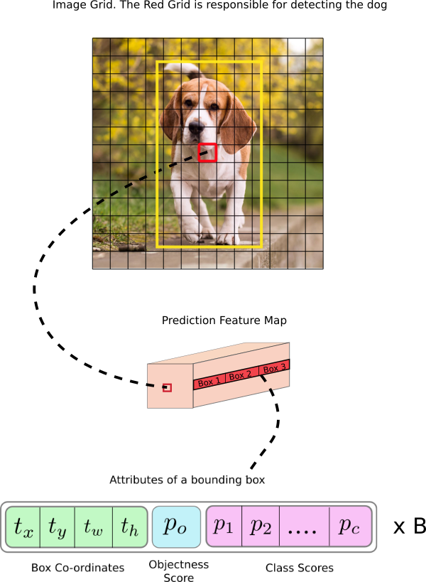
对于一个检测结果,它的信息维度为85,其中前5个数值表示为 (Cx, Cy, w, h, score),坐标是网络输入图像中的坐标,分类结果表示此处为前景区域的概率, 后面的80位代表目标归属于80分类中每一类的概率

锚点有三组, 即代表在网格的每一个位置处, 需要预测三个结果, 即 255=3*85, 这解释了特征图通道数为何为255

这里写图片描述

通过根据函数传入的输入信息, 算法首先将输入划分为13*13的网格, 步长为32, 正好可以完成到输入图像上(416=13*32)的映射

检测输出的每一项=5+classes
将锚点尺寸/stride 得到了在特征图上对应的大小

为了方便对每一个预测位置回归,需要对数据存储格式进行调整

调整之后, 先进行了

预测目标中心坐标的的偏移通过回归(sigmoid)来做,他将结果限制在(0,1)之间,是的中心不会偏移出当前网格
是否为前景目标也同样用的回归

因为先计算为中心坐标偏移量, 还需加上其在网格中位置坐标, 这样才是其在网格中的真正结果

对于宽和高预测, 这里采用exp(x)变换后得到的缩放因子乘以锚点宽高得到

这样得到了最终的坐标结果( Cx,Cy, w, h)是对应于网格中的结果, 需要乘以步长得到其在输入图像(416*416)中的位置,然后返回, 返回的结果格式为[1, ?, 85]

扩展补充:
对于尺寸为416×416的图像，YOLO V3 模型通过三个检测层预测（（52×52）+（26×26）+ 13×13））×3 = 10647个边界框。但是，在我们的示例中，只有一个物体–一只狗, 我们如何将检测结果从10647减少到1？此时用到了nms非极大值抑制, 它会剔除预测结果中位置重合过高的结果.