使用PyTorch从零开始实现YOLO-V3目标检测算法 (三)
这是从零开始实现YOLO v3检测器的教程的第3部分。第二部分中,我们实现了 YOLO 架构中使用的层。这部分,我们计划用 PyTorch 实现 YOLO 网络架构,这样我们就能生成给定图像的输出了。
我们的目标是设计网络的前向传播
本教程使用的代码需要运行在 Python 3.5 和 PyTorch 0.4 版本之上。它可以在这个Github仓库中找到。
本教程分为5个部分:
- 第1部分:了解YOLO如何工作
- 第2部分:创建网络结构
- 第3部分:实现网络的前向传播
- 第4部分:对象置信度阈值和非最大抑制
- 第5部分:设计输入和输出管道
准备
- 阅读本教程前两部分;
- PyTorch 基础知识,包括如何使用 nn.Module、nn.Sequential 和 torch.nn.parameter 创建自定义架构;
- PyTorch 中处理图像。
定义网络
如前所述,我们使用 nn.Module 在 PyTorch 中构建自定义架构。这里,我们可以为检测器定义一个网络。在 darknet.py 文件中,我们添加了以下类别:
class Darknet(nn.Module):
    def __init__(self, cfgfile):
        super(Darknet, self).__init__()
        self.blocks = parse_cfg(cfgfile)
        self.net_info, self.module_list = create_modules(self.blocks)
这里,我们对 nn.Module 类别进行子分类,并将我们的类别命名为 Darknet。我们用 members、blocks、net_info 和 module_list 对网络进行初始化。
实现网络前向传播
该网络的前向传播通过覆写 nn.Module 类别的 forward 方法而实现。
forward 主要有两个目的。一,计算输出;二,尽早处理的方式转换输出检测特征图(例如转换之后,这些不同尺度的检测图就能够串联,不然会因为不同维度不可能实现串联)。
    def forward(self, x, CUDA):
        detections = []
        modules = self.blocks[1:]
        outputs = {}  # We cache the outputs for the route layer
forward 函数有三个参数:self、输入 x 和 CUDA(如果是 true,则使用 GPU 来加速前向传播)。
这里,我们迭代 self.block[1:] 而不是 self.blocks,因为 self.blocks 的第一个元素是一个 net 块,它不属于前向传播。
由于路由层和捷径层需要之前层的输出特征图,我们在字典 outputs 中缓存每个层的输出特征图。关键在于层的索引,且值对应特征图。
正如 create_module 函数中的案例,我们现在迭代 module_list,它包含了网络的模块。需要注意的是这些模块是以在配置文件中相同的顺序添加的。这意味着,我们可以简单地让输入通过每个模块来得到输出。
        write = 0
        for i in range(len(modules)):
            module_type = (modules[i]["type"])
如果该模块是一个卷积层或上采样层,那么前向传播应该按如下方式工作:
            if module_type == "convolutional" or module_type == "upsample":
                x = self.module_list[i](x)
                outputs[i] = x
如果你查看路由层的代码,我们必须说明两个案例(正如第二部分中所描述的)。对于第一个案例,我们必须使用 torch.cat 函数将两个特征图级联起来,第二个参数设为 1。这是因为我们希望将特征图沿深度级联起来。(在 PyTorch 中,卷积层的输入和输出的格式为`B X C X H X W。深度对应通道维度)
            elif module_type == "route":
                layers = modules[i]["layers"]
                layers = [int(a) for a in layers]

                if (layers[0]) > 0:
                    layers[0] = layers[0] - i

                if len(layers) == 1:
                    x = outputs[i + (layers[0])]

                else:
                    if (layers[1]) > 0:
                        layers[1] = layers[1] - i

                    map1 = outputs[i + layers[0]]
                    map2 = outputs[i + layers[1]]

                    x = torch.cat((map1, map2), 1)
                outputs[i] = x
            elif module_type == "shortcut":
                from_ = int(modules[i]["from"])
                x = outputs[i - 1] + outputs[i + from_]
                outputs[i] = x
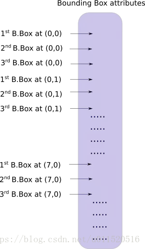
YOLO 的输出是一个卷积特征图,包含沿特征图深度的边界框属性。边界框属性由彼此堆叠的单元格预测得出。因此,如果你需要在 (5,6) 处访问单元格的第二个边框,那么你需要通过 map[5,6, (5+C): 2*(5+C)] 将其编入索引。这种格式对于输出处理过程(例如通过目标置信度进行阈值处理、添加对中心的网格偏移、应用锚点等)很不方便。
另一个问题是由于检测是在三个尺度上进行的,预测图的维度将是不同的。虽然三个特征图的维度不同,但对它们执行的输出处理过程是相似的。如果能在单个张量而不是三个单独张量上执行这些运算,就太好了。
为了解决这些问题,我们引入了函数 predict_transform。
函数 predict_transform 在文件 util.py 中,我们在 Darknet 类别的 forward 中使用该函数时,将导入该函数。
在 util.py 顶部添加导入项:
from __future__ import division

import torch
import torch.nn as nn
import torch.nn.functional as F
from torch.autograd import Variable
import numpy as np
import cv2
import matplotlib.pyplot as plt
predict_transform 使用 5 个参数:prediction(我们的输出)、inp_dim(输入图像的维度)、anchors、num_classes、CUDA flag(可选)。
def predict_transform(prediction, inp_dim, anchors, num_classes, CUDA=True):predict_transform 函数把检测特征图转换成二维张量,张量的每一行对应边界框的属性,如下所示:
上述变换所使用的代码:
    batch_size = prediction.size(0)
    stride = inp_dim // prediction.size(2)
    grid_size = inp_dim // stride
    bbox_attrs = 5 + num_classes
    num_anchors = len(anchors)

    prediction = prediction.view(batch_size, bbox_attrs * num_anchors, grid_size * grid_size)
    prediction = prediction.transpose(1, 2).contiguous()
    prediction = prediction.view(batch_size, grid_size * grid_size * num_anchors, bbox_attrs)
锚点的维度与 net 块的 height 和 width 属性一致。这些属性描述了输入图像的维度,比检测图的规模大(二者之商即是步幅)。因此,我们必须使用检测特征图的步幅分割锚点。
anchors = [(a[0] / stride, a[1] / stride) for a in anchors]现在,我们需要根据第一部分讨论的公式变换输出。
对 (x,y) 坐标和 objectness 分数执行 Sigmoid 函数操作。
    # Sigmoid the  centre_X, centre_Y. and object confidencce
    prediction[:, :, 0] = torch.sigmoid(prediction[:, :, 0])
    prediction[:, :, 1] = torch.sigmoid(prediction[:, :, 1])
    prediction[:, :, 4] = torch.sigmoid(prediction[:, :, 4])
将网格偏移添加到中心坐标预测中:
    # Add the center offsets
    grid_len = np.arange(grid_size)
    a, b = np.meshgrid(grid_len, grid_len)

    x_offset = torch.FloatTensor(a).view(-1, 1)
    y_offset = torch.FloatTensor(b).view(-1, 1)

    if CUDA:
        x_offset = x_offset.cuda()
        y_offset = y_offset.cuda()

    x_y_offset = torch.cat((x_offset, y_offset), 1).repeat(1, num_anchors).view(-1, 2).unsqueeze(0)

    prediction[:, :, :2] += x_y_offset
将锚点应用到边界框维度中:
    # log space transform height and the width
    anchors = torch.FloatTensor(anchors)

    if CUDA:
        anchors = anchors.cuda()

    anchors = anchors.repeat(grid_size * grid_size, 1).unsqueeze(0)
    prediction[:, :, 2:4] = torch.exp(prediction[:, :, 2:4]) * anchors
将 sigmoid 激活函数应用到类别分数中:
    # Softmax the class scores
    prediction[:, :, 5: 5 + num_classes] = torch.sigmoid((prediction[:, :, 5: 5 + num_classes]))
最后,我们要将检测图的大小调整到与输入图像大小一致。边界框属性根据特征图的大小而定(如 13 x 13)。如果输入图像大小是 416 x 416,那么我们将属性乘 32,或乘 stride 变量。
     prediction[:, :, :4] *= stride
    return prediction
测试前向传播
下面的函数将创建一个伪造的输入,我们可以将该输入传入我们的网络。在写该函数之前,我们可以使用以下命令行将这张图像保存到工作目录:
wget https://github.com/ayooshkathuria/pytorch-yolo-v3/raw/master/dog-cycle-car.png现在,在 darknet.py 定义以下函数:
def get_test_input():
    img = cv2.imread("img/dog-cycle-car.png")
    img = cv2.resize(img, (416, 416))
    img_ = img[:, :, ::-1].transpose((2, 0, 1))
    img_ = img_[np.newaxis, :, :, :] / 255.0
    img_ = torch.from_numpy(img_).float()
    img_ = Variable(img_)
    return img_
我们需要键入以下代码:
if __name__ == '__main__':
    model = Darknet("cfg/yolov3.cfg")
    inp = get_test_input()
    pred = model(inp, CUDA=False)
    print(pred)
有如下输出:
tensor([[[  17.5844,   18.1302,  134.9722,  ...,    0.4607,
             0.4430,    0.4889],
         [  18.1917,   17.6481,  149.9582,  ...,    0.5039,
             0.4429,    0.5111],
         [  15.1416,   16.2071,  373.7682,  ...,    0.4900,
             0.5141,    0.4745],
         ...,
         [ 411.9227,  412.1999,    8.4361,  ...,    0.4819,
             0.5525,    0.5044],
         [ 411.9741,  412.1269,   17.2431,  ...,    0.5031,
             0.4782,    0.5624],
         [ 411.8647,  411.5638,   35.2134,  ...,    0.4478,
             0.5120,    0.4918]]]
torch.Size([1, 10647, 85])
张量的形状为 1×10647×85,第一个维度为批量大小,这里我们只使用了单张图像。对于批量中的图像,我们会有一个 100647×85 的表,它的每一行表示一个边界框(4 个边界框属性、1 个 objectness 分数和 80 个类别分数)。
现在,我们的网络有随机权重,并且不会输出正确的类别。我们需要为网络加载权重文件,因此可以利用官方权重文件。
下载权重文件并放入检测器目录下,我们可以直接使用命令行下载:
wget https://pjreddie.com/media/files/yolov3.weights官方的权重文件是一个二进制文件,它以序列方式储存神经网络权重。
我们必须小心地读取权重,因为权重只是以浮点形式储存,没有其它信息能告诉我们到底它们属于哪一层。所以如果读取错误,那么很可能权重加载就全错了,模型也完全不能用。因此,只阅读浮点数,无法区别权重属于哪一层。因此,我们必须了解权重是如何存储的。
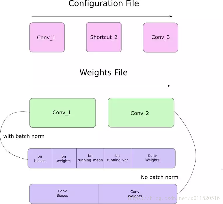
首先,权重只属于两种类型的层,即批归一化层(batch norm layer)和卷积层。这些层的权重储存顺序和配置文件中定义层级的顺序完全相同。所以,如果一个 convolutional 后面跟随着 shortcut 块,而 shortcut 连接了另一个 convolutional 块,则你会期望文件包含了先前 convolutional 块的权重,其后则是后者的权重。
当批归一化层出现在卷积模块中时,它是不带有偏置项的。然而,当卷积模块不存在批归一化,则偏置项的「权重」就会从文件中读取。下图展示了权重是如何储存的。
我们写一个函数来加载权重,它是 Darknet 类的成员函数。它使用 self 以外的一个参数作为权重文件的路径。
def load_weights(self, weightfile):第一个 160 比特的权重文件保存了 5 个 int32 值,它们构成了文件的标头。
        # Open the weights file
        fp = open(weightfile, "rb")

        # The first 4 values are header information
        # 1. Major version number
        # 2. Minor Version Number
        # 3. Subversion number
        # 4. IMages seen
        header = np.fromfile(fp, dtype=np.int32, count=5)
        self.header = torch.from_numpy(header)
        self.seen = self.header[3]
之后的比特代表权重,按上述顺序排列。权重被保存为 float32 或 32 位浮点数。我们来加载 np.ndarray 中的剩余权重。
        # The rest of the values are the weights
        # Let's load them up
        weights = np.fromfile(fp, dtype=np.float32)
现在,我们循环地加载权重文件到网络的模块上。
        ptr = 0
        for i in range(len(self.module_list)):
            module_type = self.blocks[i + 1]["type"]

            if module_type == "convolutional":
model = self.module_list[i]
try:
batch_normalize = int(self.blocks[i + 1]["batch_normalize"])
except:
batch_normalize = 0
conv = model[0]
我们保持一个称为 ptr 的变量来追踪我们在权重数组中的位置。现在,如果 batch_normalize 检查结果是 True,则我们按以下方式加载权重:
                if (batch_normalize):
                    bn = model[1]

                    # Get the number of weights of Batch Norm Layer
                    num_bn_biases = bn.bias.numel()

                    # Load the weights
                    bn_biases = torch.from_numpy(weights[ptr:ptr + num_bn_biases])
                    ptr += num_bn_biases

                    bn_weights = torch.from_numpy(weights[ptr: ptr + num_bn_biases])
                    ptr += num_bn_biases

                    bn_running_mean = torch.from_numpy(weights[ptr: ptr + num_bn_biases])
                    ptr += num_bn_biases

                    bn_running_var = torch.from_numpy(weights[ptr: ptr + num_bn_biases])
                    ptr += num_bn_biases

                    # Cast the loaded weights into dims of model weights.
                    bn_biases = bn_biases.view_as(bn.bias.data)
                    bn_weights = bn_weights.view_as(bn.weight.data)
                    bn_running_mean = bn_running_mean.view_as(bn.running_mean)
                    bn_running_var = bn_running_var.view_as(bn.running_var)

                    # Copy the data to model
                    bn.bias.data.copy_(bn_biases)
                    bn.weight.data.copy_(bn_weights)
                    bn.running_mean.copy_(bn_running_mean)
                    bn.running_var.copy_(bn_running_var)
如果 batch_normalize 的检查结果不是 True,只需要加载卷积层的偏置项。
                else:
                    # Number of biases
                    num_biases = conv.bias.numel()

                    # Load the weights
                    conv_biases = torch.from_numpy(weights[ptr: ptr + num_biases])
                    ptr = ptr + num_biases

                    # reshape the loaded weights according to the dims of the model weights
                    conv_biases = conv_biases.view_as(conv.bias.data)

                    # Finally copy the data
                    conv.bias.data.copy_(conv_biases)
最后,我们加载卷积层的权重。
                # Let us load the weights for the Convolutional layers
                num_weights = conv.weight.numel()

                # Do the same as above for weights
                conv_weights = torch.from_numpy(weights[ptr:ptr + num_weights])
                ptr = ptr + num_weights

                conv_weights = conv_weights.view_as(conv.weight.data)
                conv.weight.data.copy_(conv_weights)
该函数的介绍到此为止,你现在可以通过调用 darknet 对象上的 load_weights 函数来加载 Darknet 对象中的权重。
model = Darknet("cfg/yolov3.cfg")
model.load_weights("yolov3.weights")
通过模型构建和权重加载,我们终于可以开始进行目标检测了。未来,我们还将介绍如何利用 objectness 置信度阈值和非极大值抑制生成最终的检测结果。