使用PyTorch从零开始实现YOLO-V3目标检测算法 (四)
这是从零开始实现YOLO v3检测器的教程的第4部分,在上一部分中,我们实现了网络的前向传播。这部分,我们计划用 非极大值抑制进行置信度阈值设置。
我们的目标是设计网络的前向传播
本教程使用的代码需要运行在 Python 3.5 和 PyTorch 0.4 版本之上。它可以在这个Github仓库中找到。
本教程分为5个部分:
- 第1部分:了解YOLO如何工作
- 第2部分:创建网络结构
- 第3部分:实现网络的前向传播
- 第4部分:对象置信度阈值和非最大抑制
- 第5部分:设计输入和输出管道
先前准备
1. 教程的前3部分
2. 关于PyTorch的基础知识,包括 使用nn.Module,nn.Sequentual,torch.nn.parameter等类创建自定一的网络结构
3. 关于Numpy的基本知识
在前面 3 部分中,我们已经构建了一个能为给定输入图像输出多个目标检测结果的模型。具体来说,我们的输出是一个形状为 B x 10647 x 85 的张量;其中 B 是指一批(batch)中图像的数量,10647 是每个图像中所预测的边界框的数量,85 是指边界框属性的数量。
然而,正如第 1 部分所述,我们必须使我们的输出满足 objectness 分数阈值和非极大值抑制(NMS),以得到后文所提到的「真实(true)」检测结果。要做到这一点,我们将在 util.py 文件中创建一个名为 write_results 的函数。
def write_results(prediction, confidence, num_classes, nms=True, nms_conf=0.4):该函数的输入为预测结果、置信度(objectness 分数阈值)、num_classes(我们这里是 80)和 nms_conf(NMS IoU 阈值)。
目标置信度阈值
我们的预测张量包含有关 B x 10647 边界框的信息。对于有低于一个阈值的 objectness 分数的每个边界框,我们将其每个属性的值(表示该边界框的一整行)都设为零。
    conf_mask = (prediction[:, :, 4] > confidence).float().unsqueeze(2)
    prediction = prediction * conf_mask
执行非极大值抑制
注:我假设你已经理解 IoU(Intersection over union)和非极大值抑制(Non-maximum suppression)的含义了。如果你还不理解,请参阅文末提供的链接。
我们现在拥有的边界框属性是由中心坐标以及边界框的高度和宽度决定的。但是,使用每个框的两个对角坐标能更轻松地计算两个框的 IoU。所以,我们可以将我们的框的 (中心 x, 中心 y, 高度, 宽度) 属性转换成 (左上角 x, 左上角 y, 右下角 x, 右下角 y)。
    box_a = prediction.new(prediction.shape)
    box_a[:, :, 0] = (prediction[:, :, 0] - prediction[:, :, 2] / 2)
    box_a[:, :, 1] = (prediction[:, :, 1] - prediction[:, :, 3] / 2)
    box_a[:, :, 2] = (prediction[:, :, 0] + prediction[:, :, 2] / 2)
    box_a[:, :, 3] = (prediction[:, :, 1] + prediction[:, :, 3] / 2)
    prediction[:, :, :4] = box_a[:, :, :4]
每张图像中的「真实」检测结果的数量可能存在差异。比如,一个大小为 3 的 batch 中有 1、2、3 这 3 张图像,它们各自有 5、2、4 个「真实」检测结果。因此,一次只能完成一张图像的置信度阈值设置和 NMS。也就是说,我们不能将所涉及的操作向量化,而且必须在预测的第一个维度(包含一个 batch 中图像的索引)上循环。
 batch_size = prediction.size(0)
    write = False
    for ind in range(batch_size):
        # select the image from the batch
        image_pred = prediction[ind]
        # confidence threshholding
        # NMS
如前所述,write 标签是用于指示我们尚未初始化输出,我们将使用一个张量来收集整个 batch 的「真实」检测结果。
进入循环后,我们再更清楚地说明一下。注意每个边界框行都有 85 个属性,其中 80 个是类别分数。此时,我们只关心有最大值的类别分数。所以,我们移除了每一行的这 80 个类别分数,并且转而增加了有最大值的类别的索引以及那一类别的类别分数。
        # Get the class having maximum score, and the index of that class
        # Get rid of num_classes softmax scores
        # Add the class index and the class score of class having maximum score
        max_conf, max_conf_score = torch.max(image_pred[:, 5:5 + num_classes], 1)
        max_conf = max_conf.float().unsqueeze(1)
        max_conf_score = max_conf_score.float().unsqueeze(1)
        seq = (image_pred[:, :5], max_conf, max_conf_score)
        image_pred = torch.cat(seq, 1)
记得我们将 object 置信度小于阈值的边界框行设为零了吗?让我们丢弃它们
# Get rid of the zero entries
        non_zero_ind = (torch.nonzero(image_pred[:, 4]))

        try:
            image_pred_ = image_pred[non_zero_ind.squeeze(), :].view(-1, 7)
        except:
            continue
其中的 try-except 模块的目的是处理无检测结果的情况。在这种情况下,我们使用 continue 来跳过对本图像的循环。
现在,让我们获取一张图像中所检测到的类别。
        # Get the various classes detected in the image
        img_classes = unique(image_pred_[:, -1])
因为同一类别可能会有多个「真实」检测结果,所以我们使用一个名叫 unique 的函数来获取任意给定图像中存在的类别。
def unique(tensor):
    tensor_np = tensor.cpu().numpy()
    unique_np = np.unique(tensor_np)
    unique_tensor = torch.from_numpy(unique_np)

    tensor_res = tensor.new(unique_tensor.shape)
    tensor_res.copy_(unique_tensor)
    return tensor_res
然后,我们按照类别执行 NMS。
        # WE will do NMS classwise
        for cls in img_classes:
一旦我们进入循环,我们要做的第一件事就是提取特定类别(用变量 cls 表示)的检测结果。
            # get the detections with one particular class
            cls_mask = image_pred_ * (image_pred_[:, -1] == cls).float().unsqueeze(1)
            class_mask_ind = torch.nonzero(cls_mask[:, -2]).squeeze()

            image_pred_class = image_pred_[class_mask_ind].view(-1, 7)

            # sort the detections such that the entry with the maximum objectness
            # confidence is at the top
            conf_sort_index = torch.sort(image_pred_class[:, 4], descending=True)[1]
            image_pred_class = image_pred_class[conf_sort_index]
            idx = image_pred_class.size(0)
现在,我们执行 NMS。
                # For each detection
                for i in range(idx):
                    # Get the IOUs of all boxes that come after the one we are looking at
                    # in the loop
                    try:
                        ious = bbox_iou(image_pred_class[i].unsqueeze(0), image_pred_class[i + 1:])
                    except ValueError:
                        break

                    except IndexError:
                        break

                    # Zero out all the detections that have IoU > treshhold
                    iou_mask = (ious < nms_conf).float().unsqueeze(1)
                    image_pred_class[i + 1:] *= iou_mask

                    # Remove the non-zero entries
                    non_zero_ind = torch.nonzero(image_pred_class[:, 4]).squeeze()
                    image_pred_class = image_pred_class[non_zero_ind].view(-1, 7)
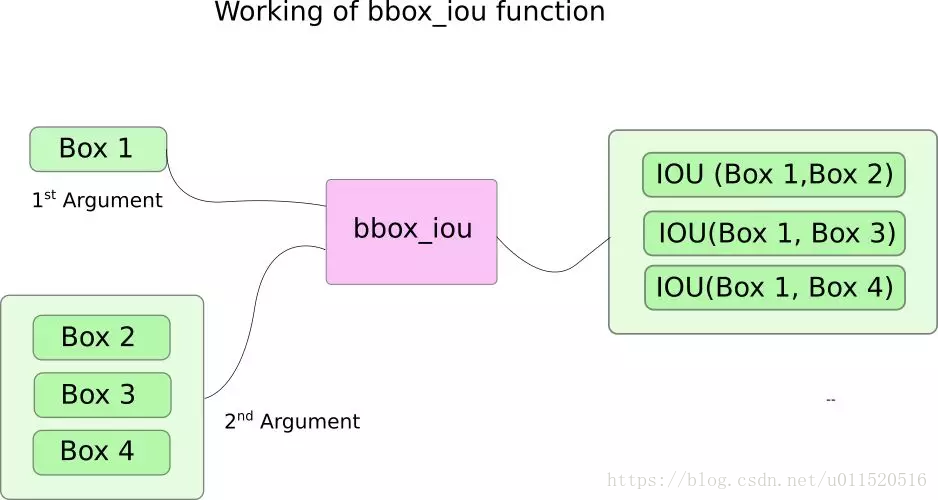
这里,我们使用了函数 bbox_iou。第一个输入是边界框行,这是由循环中的变量 i 索引的。bbox_iou 的第二个输入是多个边界框行构成的张量。bbox_iou 函数的输出是一个张量,其中包含通过第一个输入代表的边界框与第二个输入中的每个边界框的 IoU。
如果我们有 2 个同样类别的边界框且它们的 IoU 大于一个阈值,那么就去掉其中类别置信度较低的那个。我们已经对边界框进行了排序,其中有更高置信度的在上面。
在循环部分,下面的代码给出了框的 IoU,其中通过 i 索引所有索引排序高于 i 的边界框。
ious = bbox_iou(image_pred_class[i].unsqueeze(0), image_pred_class[i + 1:])每次迭代时,如果有边界框的索引大于 i 且有大于阈值 nms_thresh 的 IoU(与索引为 i 的框),那么就去掉那个特定的框。
                    # Zero out all the detections that have IoU > treshhold
                    iou_mask = (ious < nms_conf).float().unsqueeze(1)
                    image_pred_class[i + 1:] *= iou_mask

                    # Remove the non-zero entries
                    non_zero_ind = torch.nonzero(image_pred_class[:, 4]).squeeze()
                    image_pred_class = image_pred_class[non_zero_ind].view(-1, 7)
还要注意,我们已经将用于计算 ious 的代码放在了一个 try-catch 模块中。这是因为这个循环在设计上是为了运行 idx 次迭代(image_pred_class 中的行数)。但是,当我们继续循环时,一些边界框可能会从 image_pred_class 移除。这意味着,即使只从 image_pred_class 中移除了一个值,我们也不能有 idx 次迭代。因此,我们可能会尝试索引一个边界之外的值(IndexError),片状的 image_pred_class[i+1:] 可能会返回一个空张量,从而指定触发 ValueError 的量。此时,我们可以确定 NMS 不能进一步移除边界框,然后跳出循环。
计算IoPU
def bbox_iou(box1, box2):
    """
    Returns the IoU of two bounding boxes


    """
    # Get the coordinates of bounding boxes
    b1_x1, b1_y1, b1_x2, b1_y2 = box1[:, 0], box1[:, 1], box1[:, 2], box1[:, 3]
    b2_x1, b2_y1, b2_x2, b2_y2 = box2[:, 0], box2[:, 1], box2[:, 2], box2[:, 3]

    # get the corrdinates of the intersection rectangle
    inter_rect_x1 = torch.max(b1_x1, b2_x1)
    inter_rect_y1 = torch.max(b1_y1, b2_y1)
    inter_rect_x2 = torch.min(b1_x2, b2_x2)
    inter_rect_y2 = torch.min(b1_y2, b2_y2)

    # Intersection area
    if torch.cuda.is_available():
        inter_area = torch.max(inter_rect_x2 - inter_rect_x1 + 1, torch.zeros(inter_rect_x2.shape).cuda()) * torch.max(
            inter_rect_y2 - inter_rect_y1 + 1, torch.zeros(inter_rect_x2.shape).cuda())
    else:
        inter_area = torch.max(inter_rect_x2 - inter_rect_x1 + 1, torch.zeros(inter_rect_x2.shape)) * torch.max(
            inter_rect_y2 - inter_rect_y1 + 1, torch.zeros(inter_rect_x2.shape))

    # Union Area
    b1_area = (b1_x2 - b1_x1 + 1) * (b1_y2 - b1_y1 + 1)
    b2_area = (b2_x2 - b2_x1 + 1) * (b2_y2 - b2_y1 + 1)

    iou = inter_area / (b1_area + b2_area - inter_area)

    return iou
写出预测
write_results 函数输出一个形状为 Dx8 的张量;其中 D 是所有图像中的「真实」检测结果,每个都用一行表示。每一个检测结果都有 8 个属性,即:该检测结果所属的 batch 中图像的索引、4 个角的坐标、objectness 分数、有最大置信度的类别的分数、该类别的索引。
如之前一样,我们没有初始化我们的输出张量,除非我们有要分配给它的检测结果。一旦其被初始化,我们就将后续的检测结果与它连接起来。我们使用 write 标签来表示张量是否初始化了。在类别上迭代的循环结束时,我们将所得到的检测结果加入到张量输出中。
            batch_ind = image_pred_class.new(image_pred_class.size(0), 1).fill_(ind)
            seq = batch_ind, image_pred_class
            if not write:
                output = torch.cat(seq, 1)
                write = True
            else:
                out = torch.cat(seq, 1)
                output = torch.cat((output, out))
在该函数结束时,我们会检查输出是否已被初始化。如果没有,就意味着在该 batch 的任意图像中都没有单个检测结果。在这种情况下,我们返回 0。
    try:
        return output
    except:
        return 0
这部分就到此为止了。在这部分结束时,我们终于有了一个张量形式的预测结果,其中以行的形式列出了每个预测。现在还剩下:创造一个从磁盘读取图像的输入流程,计算预测结果,在图像上绘制边界框,然后展示 / 写入这些图像。这是下一部分要介绍的内容。