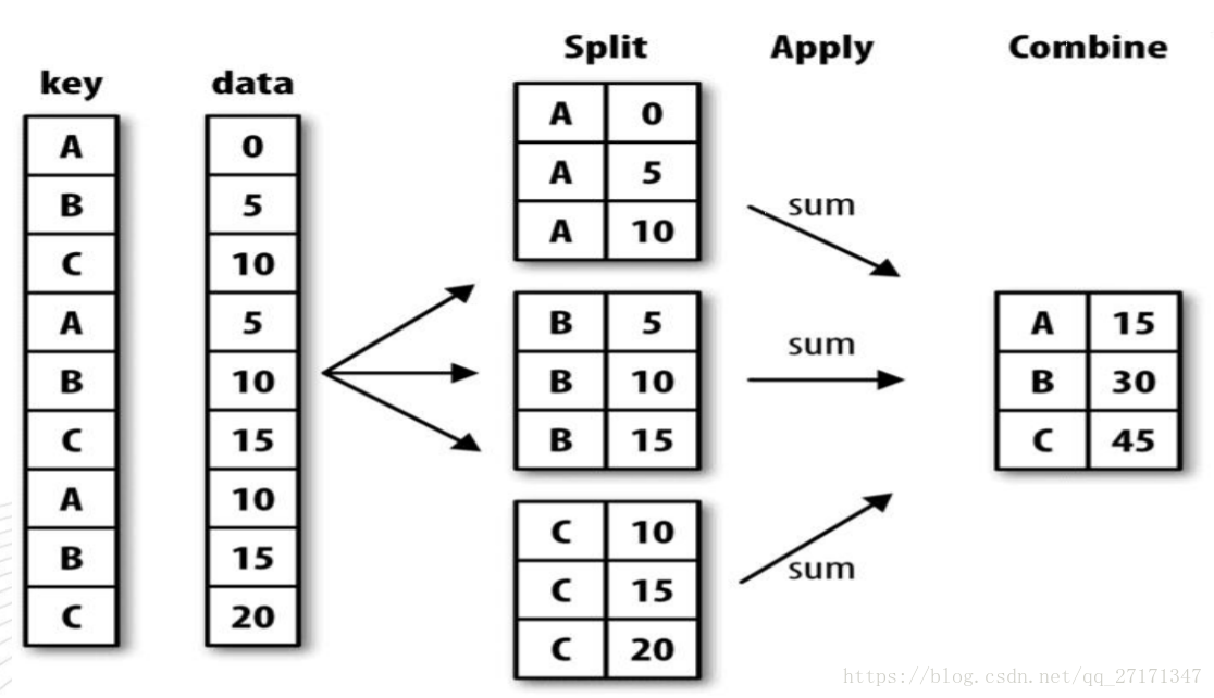
1 数据分组 - groupby()
from pandas import DataFrame,Series
import pandas as pd
import numpy as np
from numpy import nan as NA
df = DataFrame({"key1":list("aabba"),
               "key2":["one","two","one","two","one"],
               "data1":np.random.randn(5),
               "data2":np.random.randn(5)})
df
.dataframe tbody tr th:only-of-type { vertical-align: middle; } .dataframe tbody tr th { vertical-align: top; } .dataframe thead th { text-align: right; }
|
data1 |
data2 |
key1 |
key2 |
| 0 |
0.008908 |
0.652712 |
a |
one |
| 1 |
0.438874 |
0.423774 |
a |
two |
| 2 |
0.299105 |
-1.279888 |
b |
one |
| 3 |
-0.191032 |
0.429504 |
b |
two |
| 4 |
-0.395208 |
0.523417 |
a |
one |
grouped = df["data1"].groupby(df["key1"])
grouped.count()
    key1
    a    3
    b    2
    Name: data1, dtype: int64
grouped.max()
    key1
    a    0.438874
    b    0.299105
    Name: data1, dtype: float64
grouped.size()
    key1
    a    3
    b    2
    Name: data1, dtype: int64
grouped.mean()
    key1
    a    0.017525
    b    0.054036
    Name: data1, dtype: float64
grouped.describe()
.dataframe tbody tr th:only-of-type { vertical-align: middle; } .dataframe tbody tr th { vertical-align: top; } .dataframe thead th { text-align: right; }
|
count |
mean |
std |
min |
25% |
50% |
75% |
max |
| key1 |
|
|
|
|
|
|
|
|
| a |
3.0 |
0.017525 |
0.417108 |
-0.395208 |
-0.193150 |
0.008908 |
0.223891 |
0.438874 |
| b |
2.0 |
0.054036 |
0.346579 |
-0.191032 |
-0.068498 |
0.054036 |
0.176571 |
0.299105 |
df
.dataframe tbody tr th:only-of-type { vertical-align: middle; } .dataframe tbody tr th { vertical-align: top; } .dataframe thead th { text-align: right; }
|
data1 |
data2 |
key1 |
key2 |
| 0 |
0.008908 |
0.652712 |
a |
one |
| 1 |
0.438874 |
0.423774 |
a |
two |
| 2 |
0.299105 |
-1.279888 |
b |
one |
| 3 |
-0.191032 |
0.429504 |
b |
two |
| 4 |
-0.395208 |
0.523417 |
a |
one |
1.1 按照多列进行分组的两种方法
grouped1 = df["data1"].groupby([df["key1"],df["key2"]])
grouped1.mean()
    key1  key2
    a     one    -0.193150
          two     0.438874
    b     one     0.299105
          two    -0.191032
    Name: data1, dtype: float64
group_all = df.groupby(["key1","key2"])
group_all["data1"].mean()
    key1  key2
    a     one    -0.193150
          two     0.438874
    b     one     0.299105
          two    -0.191032
    Name: data1, dtype: float64
group_all["data2"].mean()
    key1  key2
    a     one     0.588065
          two     0.423774
    b     one    -1.279888
          two     0.429504
    Name: data2, dtype: float64
df
.dataframe tbody tr th:only-of-type { vertical-align: middle; } .dataframe tbody tr th { vertical-align: top; } .dataframe thead th { text-align: right; }
|
data1 |
data2 |
key1 |
key2 |
| 0 |
0.008908 |
0.652712 |
a |
one |
| 1 |
0.438874 |
0.423774 |
a |
two |
| 2 |
0.299105 |
-1.279888 |
b |
one |
| 3 |
-0.191032 |
0.429504 |
b |
two |
| 4 |
-0.395208 |
0.523417 |
a |
one |
group_key1 = df.groupby(["key1"])
1.2 对分组进行迭代
for name,group in group_key1:
print("组别:",name)
print("数据:\n",group)
    组别: a
    数据:
           data1     data2 key1 key2
    0  0.008908  0.652712    a  one
    1  0.438874  0.423774    a  two
    4 -0.395208  0.523417    a  one
    组别: b
    数据:
           data1     data2 key1 key2
    2  0.299105 -1.279888    b  one
    3 -0.191032  0.429504    b  two
1.3 将列数据按照数据类型进行分组
df
.dataframe tbody tr th:only-of-type { vertical-align: middle; } .dataframe tbody tr th { vertical-align: top; } .dataframe thead th { text-align: right; }
|
data1 |
data2 |
key1 |
key2 |
| 0 |
0.008908 |
0.652712 |
a |
one |
| 1 |
0.438874 |
0.423774 |
a |
two |
| 2 |
0.299105 |
-1.279888 |
b |
one |
| 3 |
-0.191032 |
0.429504 |
b |
two |
| 4 |
-0.395208 |
0.523417 |
a |
one |
df.dtypes
    data1    float64
    data2    float64
    key1      object
    key2      object
    dtype: object
group_types = df.groupby(df.dtypes,axis=1)
for name,group in group_types:
    print("组别:",name)
    print("数据:\n",group)
    组别: float64
    数据:
           data1     data2
    0  0.008908  0.652712
    1  0.438874  0.423774
    2  0.299105 -1.279888
    3 -0.191032  0.429504
    4 -0.395208  0.523417
    组别: object
    数据:
       key1 key2
    0    a  one
    1    a  two
    2    b  one
    3    b  two
    4    a  one
1.4 通过字典或者Series对DataFrame数据进行分组
people = DataFrame(np.random.randn(5,5),
                  columns=list("abcde"),
                  index=["Joe","Jack","Rose","Tom","Jerry"])
people
.dataframe tbody tr th:only-of-type { vertical-align: middle; } .dataframe tbody tr th { vertical-align: top; } .dataframe thead th { text-align: right; }
|
a |
b |
c |
d |
e |
| Joe |
1.147082 |
0.053921 |
0.182772 |
-0.885232 |
1.486824 |
| Jack |
-1.020139 |
-0.818716 |
2.464176 |
-0.323069 |
0.987470 |
| Rose |
-0.478689 |
-0.025389 |
1.585679 |
-0.555187 |
0.075537 |
| Tom |
0.357304 |
1.033158 |
0.589091 |
-0.003958 |
-0.659374 |
| Jerry |
1.617607 |
-1.523480 |
-0.449035 |
-0.784486 |
-2.736335 |
people.ix[2:3,["b","c"]] = NA
people
.dataframe tbody tr th:only-of-type { vertical-align: middle; } .dataframe tbody tr th { vertical-align: top; } .dataframe thead th { text-align: right; }
|
a |
b |
c |
d |
e |
| Joe |
1.147082 |
0.053921 |
0.182772 |
-0.885232 |
1.486824 |
| Jack |
-1.020139 |
-0.818716 |
2.464176 |
-0.323069 |
0.987470 |
| Rose |
-0.478689 |
NaN |
NaN |
-0.555187 |
0.075537 |
| Tom |
0.357304 |
1.033158 |
0.589091 |
-0.003958 |
-0.659374 |
| Jerry |
1.617607 |
-1.523480 |
-0.449035 |
-0.784486 |
-2.736335 |
mapping = {"a":"red",
          "b":"red",
          "c":"blue",
          "d":"blue",
          "e":"red",
          "f":"orange"}
group_dict = people.groupby(mapping,axis=1)
group_dict.count()
.dataframe tbody tr th:only-of-type { vertical-align: middle; } .dataframe tbody tr th { vertical-align: top; } .dataframe thead th { text-align: right; }
|
blue |
red |
| Joe |
2 |
3 |
| Jack |
2 |
3 |
| Rose |
1 |
2 |
| Tom |
2 |
3 |
| Jerry |
2 |
3 |
group_dict.sum()
.dataframe tbody tr th:only-of-type { vertical-align: middle; } .dataframe tbody tr th { vertical-align: top; } .dataframe thead th { text-align: right; }
|
blue |
red |
| Joe |
-0.702460 |
2.687828 |
| Jack |
2.141107 |
-0.851385 |
| Rose |
-0.555187 |
-0.403153 |
| Tom |
0.585133 |
0.731088 |
| Jerry |
-1.233521 |
-2.642209 |
group_dict.mean()
.dataframe tbody tr th:only-of-type { vertical-align: middle; } .dataframe tbody tr th { vertical-align: top; } .dataframe thead th { text-align: right; }
|
blue |
red |
| Joe |
-0.351230 |
0.895943 |
| Jack |
1.070553 |
-0.283795 |
| Rose |
-0.555187 |
-0.201576 |
| Tom |
0.292566 |
0.243696 |
| Jerry |
-0.616761 |
-0.880736 |
2 数据聚合
2.1 分组结果的内置聚合函数
- df_obj5.groupby(‘key1’).sum()
- df_obj5.groupby(‘key1’).max()
- df_obj5.groupby(‘key1’).min()
- df_obj5.groupby(‘key1’).mean()
- df_obj5.groupby(‘key1’).size()
- df_obj5.groupby(‘key1’).count()
- df_obj5.groupby(‘key1’).describe()
| 函数名 |
说明 |
| count |
分组中非NA值的数量 |
| sum |
非NA值的和 |
| mean |
非NA值的算术平均数 |
| median |
非NA值的算数中位数 |
| std,var |
无偏标准差和方差 |
| min,max |
非NA值的最小最大值 |
| prod |
非NA值的积 |
| first,last |
第一个和最后一个非NA值 |
dict_obj = {'key1' : ['a' , 'b' , 'a' , 'b' , 'a' , 'b' , 'a' , 'a'],
'key2' : ['one' , 'one' , 'two' , 'three' ,'two' , 'two' , 'one' , 'three'],
'data1': np.random.randint(1,10, 8),
'data2': np.random.randint(1,10, 8)}
df_dict = DataFrame(dict_obj)
df_dict
.dataframe tbody tr th:only-of-type { vertical-align: middle; } .dataframe tbody tr th { vertical-align: top; } .dataframe thead th { text-align: right; }
|
data1 |
data2 |
key1 |
key2 |
| 0 |
4 |
5 |
a |
one |
| 1 |
2 |
9 |
b |
one |
| 2 |
8 |
2 |
a |
two |
| 3 |
7 |
7 |
b |
three |
| 4 |
3 |
4 |
a |
two |
| 5 |
4 |
6 |
b |
two |
| 6 |
3 |
5 |
a |
one |
| 7 |
5 |
7 |
a |
three |
grouped = df_dict.groupby("key1")
grouped.count()
.dataframe tbody tr th:only-of-type { vertical-align: middle; } .dataframe tbody tr th { vertical-align: top; } .dataframe thead th { text-align: right; }
|
data1 |
data2 |
key2 |
| key1 |
|
|
|
| a |
5 |
5 |
5 |
| b |
3 |
3 |
3 |
grouped.sum()
.dataframe tbody tr th:only-of-type { vertical-align: middle; } .dataframe tbody tr th { vertical-align: top; } .dataframe thead th { text-align: right; }
|
data1 |
data2 |
| key1 |
|
|
| a |
23 |
23 |
| b |
13 |
22 |
df_dict
.dataframe tbody tr th:only-of-type { vertical-align: middle; } .dataframe tbody tr th { vertical-align: top; } .dataframe thead th { text-align: right; }
|
data1 |
data2 |
key1 |
key2 |
| 0 |
4 |
5 |
a |
one |
| 1 |
2 |
9 |
b |
one |
| 2 |
8 |
2 |
a |
two |
| 3 |
7 |
7 |
b |
three |
| 4 |
3 |
4 |
a |
two |
| 5 |
4 |
6 |
b |
two |
| 6 |
3 |
5 |
a |
one |
| 7 |
5 |
7 |
a |
three |
grouped = df_dict.groupby("key1")
grouped
<pandas.core.groupby.DataFrameGroupBy object at 0x00000207EA25FBE0>
2.2 自定义聚合函数
def peak_range(group):
return group.max()-group.min()
grouped.agg(lambda group : group.max()-group.min())
.dataframe tbody tr th:only-of-type { vertical-align: middle; } .dataframe tbody tr th { vertical-align: top; } .dataframe thead th { text-align: right; }
|
data1 |
data2 |
| key1 |
|
|
| a |
5 |
5 |
| b |
5 |
3 |
grouped.agg(["mean","std","count",peak_range])
.dataframe tbody tr th:only-of-type { vertical-align: middle; } .dataframe tbody tr th { vertical-align: top; } .dataframe thead tr th { text-align: left; } .dataframe thead tr:last-of-type th { text-align: right; }
|
data1 |
data2 |
|
mean |
std |
count |
peak_range |
mean |
std |
count |
peak_range |
| key1 |
|
|
|
|
|
|
|
|
| a |
4.600000 |
2.073644 |
5 |
5 |
4.600000 |
1.816590 |
5 |
5 |
| b |
4.333333 |
2.516611 |
3 |
5 |
7.333333 |
1.527525 |
3 |
3 |
grouped.agg(["mean","std","count",("ptp",peak_range)])
.dataframe tbody tr th:only-of-type { vertical-align: middle; } .dataframe tbody tr th { vertical-align: top; } .dataframe thead tr th { text-align: left; } .dataframe thead tr:last-of-type th { text-align: right; }
|
data1 |
data2 |
|
mean |
std |
count |
ptp |
mean |
std |
count |
ptp |
| key1 |
|
|
|
|
|
|
|
|
| a |
4.600000 |
2.073644 |
5 |
5 |
4.600000 |
1.816590 |
5 |
5 |
| b |
4.333333 |
2.516611 |
3 |
5 |
7.333333 |
1.527525 |
3 |
3 |
for name,group in grouped:
print("组别:",name)
print("数据:\n",group)
    组别: a
    数据:
        data1  data2 key1   key2
    0      4      5    a    one
    2      8      2    a    two
    4      3      4    a    two
    6      3      5    a    one
    7      5      7    a  three
    组别: b
    数据:
        data1  data2 key1   key2
    1      2      9    b    one
    3      7      7    b  three
    5      4      6    b    two
func_type = {"data1":"mean",
"data2":"sum"}
grouped.agg(func_type)
.dataframe tbody tr th:only-of-type { vertical-align: middle; } .dataframe tbody tr th { vertical-align: top; } .dataframe thead th { text-align: right; }
|
data1 |
data2 |
| key1 |
|
|
| a |
4.600000 |
23 |
| b |
4.333333 |
22 |
df = pd.DataFrame({'books':['bk1' , 'bk1' , 'bk1' , 'bk2' , 'bk2' , 'bk3'],
'price': [12,12,12,15,15,17]})
df
.dataframe tbody tr th:only-of-type { vertical-align: middle; } .dataframe tbody tr th { vertical-align: top; } .dataframe thead th { text-align: right; }
|
books |
price |
| 0 |
bk1 |
12 |
| 1 |
bk1 |
12 |
| 2 |
bk1 |
12 |
| 3 |
bk2 |
15 |
| 4 |
bk2 |
15 |
| 5 |
bk3 |
17 |
book_group = df.groupby("books",as_index=True)
book_group.sum()
.dataframe tbody tr th:only-of-type { vertical-align: middle; } .dataframe tbody tr th { vertical-align: top; } .dataframe thead th { text-align: right; }
|
price |
| books |
|
| bk1 |
36 |
| bk2 |
30 |
| bk3 |
17 |
2.3 apply函数
tips = pd.read_csv("data/tips.csv")
tips.head(5)
.dataframe tbody tr th:only-of-type { vertical-align: middle; } .dataframe tbody tr th { vertical-align: top; } .dataframe thead th { text-align: right; }
|
total_bill |
tip |
smoker |
day |
time |
size |
| 0 |
16.99 |
1.01 |
No |
Sun |
Dinner |
2 |
| 1 |
10.34 |
1.66 |
No |
Sun |
Dinner |
3 |
| 2 |
21.01 |
3.50 |
No |
Sun |
Dinner |
3 |
| 3 |
23.68 |
3.31 |
No |
Sun |
Dinner |
2 |
| 4 |
24.59 |
3.61 |
No |
Sun |
Dinner |
4 |
tips["tip_pct"] = tips["tip"]/tips["total_bill"]
tips.head(5)
.dataframe tbody tr th:only-of-type { vertical-align: middle; } .dataframe tbody tr th { vertical-align: top; } .dataframe thead th { text-align: right; }
|
total_bill |
tip |
smoker |
day |
time |
size |
tip_pct |
| 0 |
16.99 |
1.01 |
No |
Sun |
Dinner |
2 |
0.059447 |
| 1 |
10.34 |
1.66 |
No |
Sun |
Dinner |
3 |
0.160542 |
| 2 |
21.01 |
3.50 |
No |
Sun |
Dinner |
3 |
0.166587 |
| 3 |
23.68 |
3.31 |
No |
Sun |
Dinner |
2 |
0.139780 |
| 4 |
24.59 |
3.61 |
No |
Sun |
Dinner |
4 |
0.146808 |
def top(df,n=5,col="tip_pct"):
return df.sort_values(by=col,ascending=True)[:n]
top(tips,n=10,col="total_bill")
.dataframe tbody tr th:only-of-type { vertical-align: middle; } .dataframe tbody tr th { vertical-align: top; } .dataframe thead th { text-align: right; }
|
total_bill |
tip |
smoker |
day |
time |
size |
tip_pct |
| 67 |
3.07 |
1.00 |
Yes |
Sat |
Dinner |
1 |
0.325733 |
| 92 |
5.75 |
1.00 |
Yes |
Fri |
Dinner |
2 |
0.173913 |
| 111 |
7.25 |
1.00 |
No |
Sat |
Dinner |
1 |
0.137931 |
| 172 |
7.25 |
5.15 |
Yes |
Sun |
Dinner |
2 |
0.710345 |
| 149 |
7.51 |
2.00 |
No |
Thur |
Lunch |
2 |
0.266312 |
| 195 |
7.56 |
1.44 |
No |
Thur |
Lunch |
2 |
0.190476 |
| 218 |
7.74 |
1.44 |
Yes |
Sat |
Dinner |
2 |
0.186047 |
| 145 |
8.35 |
1.50 |
No |
Thur |
Lunch |
2 |
0.179641 |
| 135 |
8.51 |
1.25 |
No |
Thur |
Lunch |
2 |
0.146886 |
| 126 |
8.52 |
1.48 |
No |
Thur |
Lunch |
2 |
0.173709 |
自定义函数利用apply应用到分组对象上
group_by_smoker.apply(top)
.dataframe tbody tr th:only-of-type { vertical-align: middle; } .dataframe tbody tr th { vertical-align: top; } .dataframe thead th { text-align: right; }
|
|
total_bill |
tip |
smoker |
day |
time |
size |
tip_pct |
| smoker |
|
|
|
|
|
|
|
|
| No |
57 |
26.41 |
1.50 |
No |
Sat |
Dinner |
2 |
0.056797 |
| 0 |
16.99 |
1.01 |
No |
Sun |
Dinner |
2 |
0.059447 |
| 48 |
28.55 |
2.05 |
No |
Sun |
Dinner |
3 |
0.071804 |
| 146 |
18.64 |
1.36 |
No |
Thur |
Lunch |
3 |
0.072961 |
| 130 |
19.08 |
1.50 |
No |
Thur |
Lunch |
2 |
0.078616 |
| Yes |
237 |
32.83 |
1.17 |
Yes |
Sat |
Dinner |
2 |
0.035638 |
| 102 |
44.30 |
2.50 |
Yes |
Sat |
Dinner |
3 |
0.056433 |
| 187 |
30.46 |
2.00 |
Yes |
Sun |
Dinner |
5 |
0.065660 |
| 210 |
30.06 |
2.00 |
Yes |
Sat |
Dinner |
3 |
0.066534 |
| 240 |
27.18 |
2.00 |
Yes |
Sat |
Dinner |
2 |
0.073584 |
tips.head(5)
tips.head(5)
.dataframe tbody tr th:only-of-type { vertical-align: middle; } .dataframe tbody tr th { vertical-align: top; } .dataframe thead th { text-align: right; }
|
total_bill |
tip |
smoker |
day |
time |
size |
tip_pct |
| 0 |
16.99 |
1.01 |
No |
Sun |
Dinner |
2 |
0.059447 |
| 1 |
10.34 |
1.66 |
No |
Sun |
Dinner |
3 |
0.160542 |
| 2 |
21.01 |
3.50 |
No |
Sun |
Dinner |
3 |
0.166587 |
| 3 |
23.68 |
3.31 |
No |
Sun |
Dinner |
2 |
0.139780 |
| 4 |
24.59 |
3.61 |
No |
Sun |
Dinner |
4 |
0.146808 |
mask = tips["smoker"] == "Yes"
smoker_data = tips[mask]
smoker_data
top(smoker_data)
.dataframe tbody tr th:only-of-type { vertical-align: middle; } .dataframe tbody tr th { vertical-align: top; } .dataframe thead th { text-align: right; }
|
total_bill |
tip |
smoker |
day |
time |
size |
tip_pct |
| 237 |
32.83 |
1.17 |
Yes |
Sat |
Dinner |
2 |
0.035638 |
| 102 |
44.30 |
2.50 |
Yes |
Sat |
Dinner |
3 |
0.056433 |
| 187 |
30.46 |
2.00 |
Yes |
Sun |
Dinner |
5 |
0.065660 |
| 210 |
30.06 |
2.00 |
Yes |
Sat |
Dinner |
3 |
0.066534 |
| 240 |
27.18 |
2.00 |
Yes |
Sat |
Dinner |
2 |
0.073584 |
mask=tips["smoker"]=="No"
none_smoker_data = tips[mask]
top(none_smoker_data)
.dataframe tbody tr th:only-of-type { vertical-align: middle; } .dataframe tbody tr th { vertical-align: top; } .dataframe thead th { text-align: right; }
|
total_bill |
tip |
smoker |
day |
time |
size |
tip_pct |
| 57 |
26.41 |
1.50 |
No |
Sat |
Dinner |
2 |
0.056797 |
| 0 |
16.99 |
1.01 |
No |
Sun |
Dinner |
2 |
0.059447 |
| 48 |
28.55 |
2.05 |
No |
Sun |
Dinner |
3 |
0.071804 |
| 146 |
18.64 |
1.36 |
No |
Thur |
Lunch |
3 |
0.072961 |
| 130 |
19.08 |
1.50 |
No |
Thur |
Lunch |
2 |
0.078616 |
tips.groupby(["smoker","day"]).apply(top,n=2,col="total_bill")
.dataframe tbody tr th:only-of-type { vertical-align: middle; } .dataframe tbody tr th { vertical-align: top; } .dataframe thead th { text-align: right; }
|
|
|
total_bill |
tip |
smoker |
day |
time |
size |
tip_pct |
| smoker |
day |
|
|
|
|
|
|
|
|
| No |
Fri |
99 |
12.46 |
1.50 |
No |
Fri |
Dinner |
2 |
0.120385 |
| 223 |
15.98 |
3.00 |
No |
Fri |
Lunch |
3 |
0.187735 |
| Sat |
111 |
7.25 |
1.00 |
No |
Sat |
Dinner |
1 |
0.137931 |
| 30 |
9.55 |
1.45 |
No |
Sat |
Dinner |
2 |
0.151832 |
| Sun |
6 |
8.77 |
2.00 |
No |
Sun |
Dinner |
2 |
0.228050 |
| 43 |
9.68 |
1.32 |
No |
Sun |
Dinner |
2 |
0.136364 |
| Thur |
149 |
7.51 |
2.00 |
No |
Thur |
Lunch |
2 |
0.266312 |
| 195 |
7.56 |
1.44 |
No |
Thur |
Lunch |
2 |
0.190476 |
| Yes |
Fri |
92 |
5.75 |
1.00 |
Yes |
Fri |
Dinner |
2 |
0.173913 |
| 222 |
8.58 |
1.92 |
Yes |
Fri |
Lunch |
1 |
0.223776 |
| Sat |
67 |
3.07 |
1.00 |
Yes |
Sat |
Dinner |
1 |
0.325733 |
| 218 |
7.74 |
1.44 |
Yes |
Sat |
Dinner |
2 |
0.186047 |
| Sun |
172 |
7.25 |
5.15 |
Yes |
Sun |
Dinner |
2 |
0.710345 |
| 178 |
9.60 |
4.00 |
Yes |
Sun |
Dinner |
2 |
0.416667 |
| Thur |
196 |
10.34 |
2.00 |
Yes |
Thur |
Lunch |
2 |
0.193424 |
| 201 |
12.74 |
2.01 |
Yes |
Thur |
Lunch |
2 |
0.157771 |
tips.groupby("smoker",group_keys=False).apply(top)
.dataframe tbody tr th:only-of-type { vertical-align: middle; } .dataframe tbody tr th { vertical-align: top; } .dataframe thead th { text-align: right; }
|
total_bill |
tip |
smoker |
day |
time |
size |
tip_pct |
| 57 |
26.41 |
1.50 |
No |
Sat |
Dinner |
2 |
0.056797 |
| 0 |
16.99 |
1.01 |
No |
Sun |
Dinner |
2 |
0.059447 |
| 48 |
28.55 |
2.05 |
No |
Sun |
Dinner |
3 |
0.071804 |
| 146 |
18.64 |
1.36 |
No |
Thur |
Lunch |
3 |
0.072961 |
| 130 |
19.08 |
1.50 |
No |
Thur |
Lunch |
2 |
0.078616 |
| 237 |
32.83 |
1.17 |
Yes |
Sat |
Dinner |
2 |
0.035638 |
| 102 |
44.30 |
2.50 |
Yes |
Sat |
Dinner |
3 |
0.056433 |
| 187 |
30.46 |
2.00 |
Yes |
Sun |
Dinner |
5 |
0.065660 |
| 210 |
30.06 |
2.00 |
Yes |
Sat |
Dinner |
3 |
0.066534 |
| 240 |
27.18 |
2.00 |
Yes |
Sat |
Dinner |
2 |
0.073584 |
2.4 分组加权平均数和相关系数
df = pd.DataFrame({'category': ['a' , 'a' , 'a' , 'a' , 'b' , 'b' , 'b' , 'b'],
                   'data': np.random.randn(8),
                   'weights': np.random.rand(8)})
df
.dataframe tbody tr th:only-of-type { vertical-align: middle; } .dataframe tbody tr th { vertical-align: top; } .dataframe thead th { text-align: right; }
|
category |
data |
weights |
| 0 |
a |
-1.837433 |
0.220477 |
| 1 |
a |
-1.572593 |
0.615787 |
| 2 |
a |
0.008959 |
0.640871 |
| 3 |
a |
1.095008 |
0.305419 |
| 4 |
b |
0.190451 |
0.290830 |
| 5 |
b |
1.201876 |
0.904729 |
| 6 |
b |
-1.125858 |
0.821191 |
| 7 |
b |
-0.946454 |
0.039222 |
grouped = df.groupby("category")
for name,group in grouped:
    print("组别:",name)
    print("数据:\n",group)
    组别: a
    数据:
       category      data   weights
    0        a -1.837433  0.220477
    1        a -1.572593  0.615787
    2        a  0.008959  0.640871
    3        a  1.095008  0.305419
    组别: b
    数据:
       category      data   weights
    4        b  0.190451  0.290830
    5        b  1.201876  0.904729
    6        b -1.125858  0.821191
    7        b -0.946454  0.039222
def getAvg(df):
    return  np.average(df["data"],weights=df["weights"])

grouped.apply(getAvg)
    category
    a   -0.579683
    b    0.088082
    dtype: float64
df
.dataframe tbody tr th:only-of-type { vertical-align: middle; } .dataframe tbody tr th { vertical-align: top; } .dataframe thead th { text-align: right; }
|
category |
data |
weights |
| 0 |
a |
-1.837433 |
0.220477 |
| 1 |
a |
-1.572593 |
0.615787 |
| 2 |
a |
0.008959 |
0.640871 |
| 3 |
a |
1.095008 |
0.305419 |
| 4 |
b |
0.190451 |
0.290830 |
| 5 |
b |
1.201876 |
0.904729 |
| 6 |
b |
-1.125858 |
0.821191 |
| 7 |
b |
-0.946454 |
0.039222 |