Mitosis Detection in Breast Cancer Histology Images with Deep Neural Networks

1，Mitosis Detection in Breast Cancer Histology Images with Deep Neural Networks

这篇文章发表在 MICCAI2013 ,文章中提出的方法在 ICPR2012 mitosis detection competition 中取得了第一名。 其中方法大致为(Fig.1)：

Fig.1
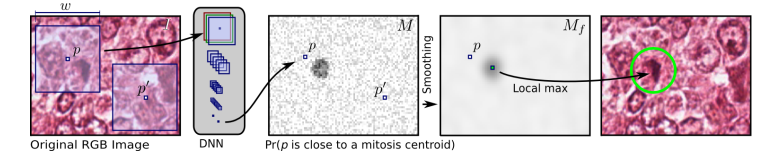
1,训练一个CNN分类器，判断以每个像素点为中心的正方形框是 mitosis 的概率。

要解决两个的问题：
1） 边界区域像素点怎么判断？
边界区域像素点的采用镜像来扩增其周围的像素点构成正方形框

2） 训练数据集的产生
 1, the mitosis class is assigned to all windows whose center pixel is closer than d = 10 pixels to the centroid of a ground-truth mitosis; all remaining windows are given the non-mitosis class. This results in a total of roughly 66000 mitosis pixels and 151 million non-mitosis pixels。
 注意到不是所有的 non-mitosis 都有意义。因为如文中所说：In contrast, the largest part of the image area is covered by background pixels far from any nucleus, whose class (non-mitosis) is quite trivial to determine. If training instances for class non-mitosis were uniformly sampled from images, most of the training effort would be wasted.

 2, 去除对训练没有价值的数据，构造更有价值的数据集。其中一种方法是 first detecting all nuclei, then classifying each nucleus separately as mitotic or non-mitotic. 而文中采用的方法不需要更多的先验知识：

1. We build a small training set Sd, which includes all 66000 mitosis instances and the same number of non-mitosis instances, uniformly sampled from the 151 million non-mitosis pixels.
2. We use Sd to briefly train a simple DNN classifier Cd. Because Cd is trained on a limited training set in which challenging non-mitosis instances are severely underrepresented, it tends to misclassify most non-mitotic nuclei as class mitosis
3. We apply Cd to all images in T1 and T2. Let D(p) denote the mitosis probability that Cd assigns to pixel p. D(p) will be large for challenging non-mitosis pixels.
4. We build the actual training set, composed by 1 million instances, which includes
   all mitosis pixels (6:6% of the training instances). The remaining 95:4% is sampled from non-mitosis pixels by assigning to each pixel p a weight D(p)

2, 求概率图 M
使用训练的模型来预测图像中每一个像素点为中心的正方形框是 mitosis 的概率，得到概率图 M 。

3, 求平滑后的概率图 $M_f$
我们期望 M 在非有丝分裂区域的值都为0，但是实际上预测出来的结果肯定不会是这样，因此需要让极值区域更加集中。于是采用文中提出的 smooth 方法：将 M 与一个以 d 个像素为半径的圆形核卷积。得到 smooth 后的概率图像 $M_f$ 。

4,选取 detections

1）先确定一个阈值 t（最优值由交叉检验产生） 。$p_m$ 表示最大像素点的位置，选取 $M_f(p_m)$ 中的最大值，判断 $M_f(p_m)$ 是否大于阈值 t ,如果大于，则进入第二步，否则选取流程结束。

2）为避免同一块区域出现多个 detection，对于 $|p-p_m|<2d,$ $M_f(p)$ <— 0 。

---

3,A Unified Framework for Tumor ProliferationScore Prediction in Breast Histopathology

This paper was accepted by the 3rd Workshop on Deep Learning in Medical Image Analysis (DLMIA 2017), MICCAI 2017.The system presented won first place in all of three tasks in Tumor Proliferation Challenge at MICCAI 2016.

1,INTRODUCTION(the same as the paper above)

This paper was submitted to CVPR2016. Here is the link .This study presents the dirst data-driven approach to characterize the severity of tumor groeth on a categorical and molecular level.,utilizing multiple biologically salient deep learning classifiers.

• dataset : Three dataset were used in this study. you can find the detailed information in this link. The primary dataset consists of 500 breast cancer cases. Each case is represented by one whole-slide image (WSI) and is annotated with a proliferation score (3 classes). The first auxiliary dataset consist of 73 images. Regions that contain mitotic figures with be marked,So it can be used train a mitosis detection model. The second suxiliary dataset consists of 148 images. Regions of interst of each image will ne marked.So it can be used to train a region of interest model.
• target : predict tumor proliferation score based on mitosis counting.

2,METHODS(Fig.3)

Fig3
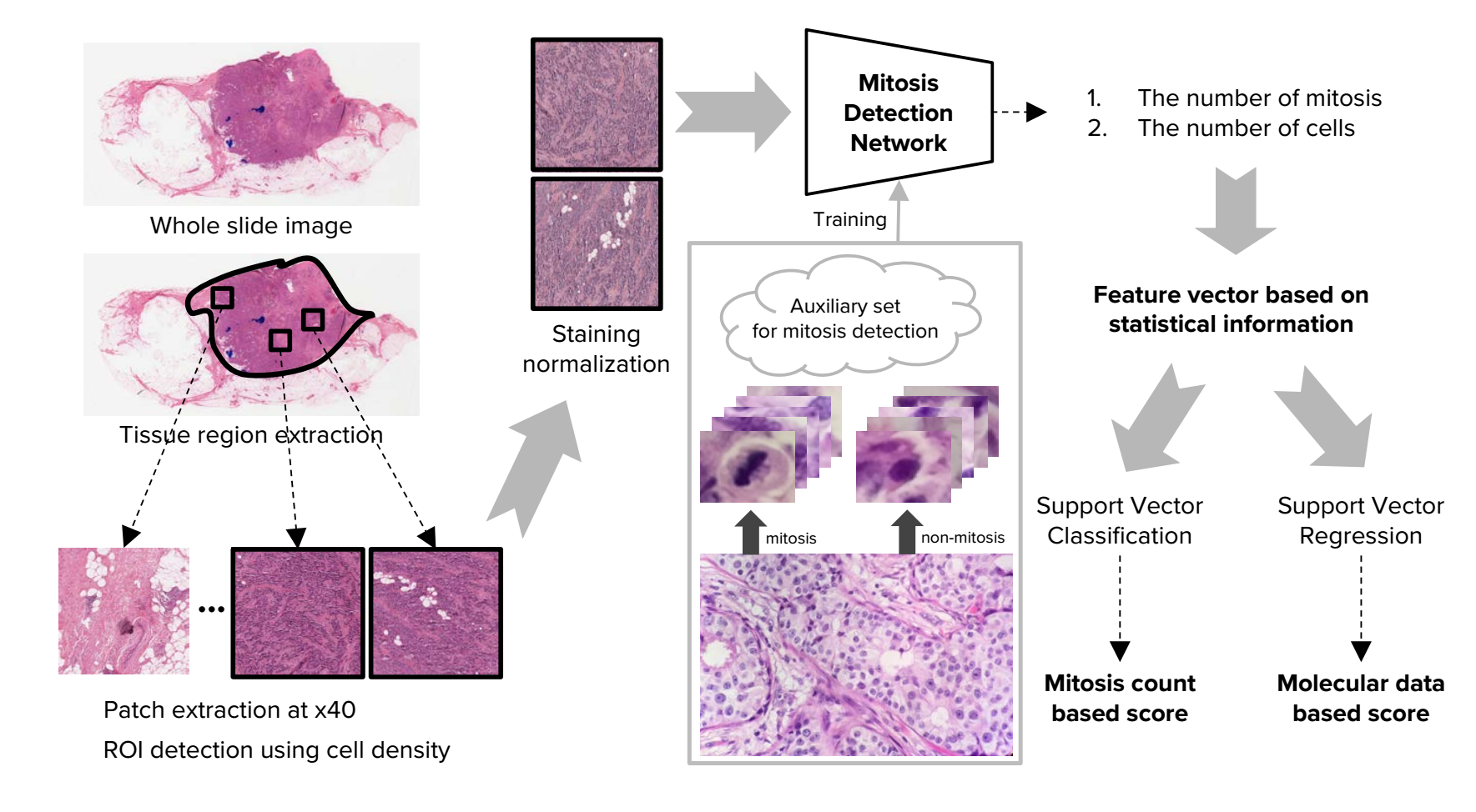
1, Whole Slide Images Handling
   1) Tisuue region and patch extraction.The size of the patches is 10HPFs.
   2) ROI detection. According to the number of cells in each patch,the top k patches are chosen as ROIs.In this paper,k equals 30.
   3) Staining normalization

2,CNN based Mitosis Detection
   1), we randomly extract 180,000 normal patches and 70,000 random translation augmented mitosis patches from the training dataset. We perform a first-pass training of the network by using this initial dataset, and perform inference with the trained network weights to extract a list of image regions that the network has identified as false positive mitoses cases. After that, we build a new, second training dataset which consists of the same ground truth mitosis samples and normal samples from before, but with an additional 100,000 normal samples (i.e., false positives) generated with random translation augmentation from the initially trained network. In total, the new dataset consists of 70,000 mitosis patches and 280,000 normal patches. In the second training step, the final detection network is trained from scratch using the new training dataset
   2), Although we train the network using small patches (i.e.,specific mitosis regions), the patches we ultimately infer on during the test phase are 10 HPFs regions sampled from WSIs, which are approximately 6000 x 6000 pixels. One way to perform prediction is to divide the ROI patch into patches of equal size to the training images, but this would incur large computation costs.
  Therefore, we convert the trained network to a fully convolutional network [10] at the inference stage, which allows our trained network to perform inference on an entire 10HPFs image with a single forward pass.However, the prediction results based on the fully convolutional network is
not identical to that of original network. We call this problem the zero padding effect. There are two reasons for the zero padding effect: (1) ResNet has a large receptive field because the depth of the network is very large. (2) The residual block in ResNet has many zero padding to retain the spatial dimension. Thus, the receptive field of the trained network includes zero padding regions as shown in Fig.4

Fig.4

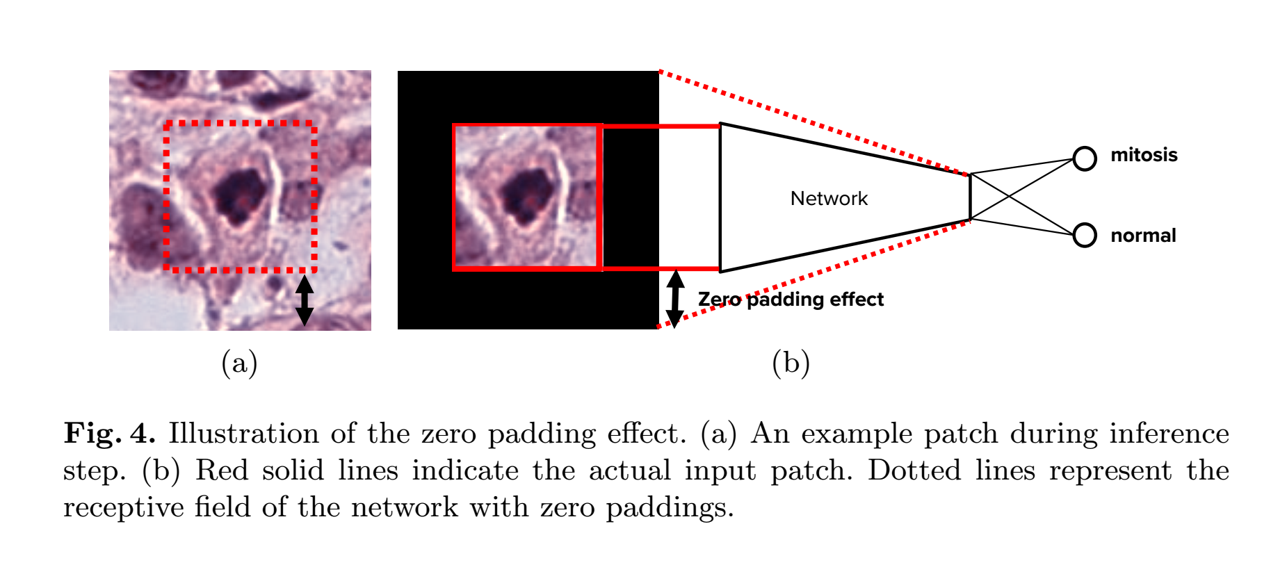
  In order to alleviate this problem, we introduce a novel architecture named largeview (L-view) model(Fig.5). Although the L-view architecture has 128 x 128 input size, in the final layer(the result is a scalar,so it is not a layer and the last layer is the layer before the result), we only use a smaller region corresponding to a 64 x 64 region in the input patch. Fig. 5 shows the L-view architecture. Only the region corresponding to this smaller region is activated at the global pooling layer. This allows the zero padding region to be ignored in the training phase and consequently solves the problem of the zero padding effect.(难点 ：将一个种input size 训练出来的FCN，应用到另外一种input size)

Fig.5
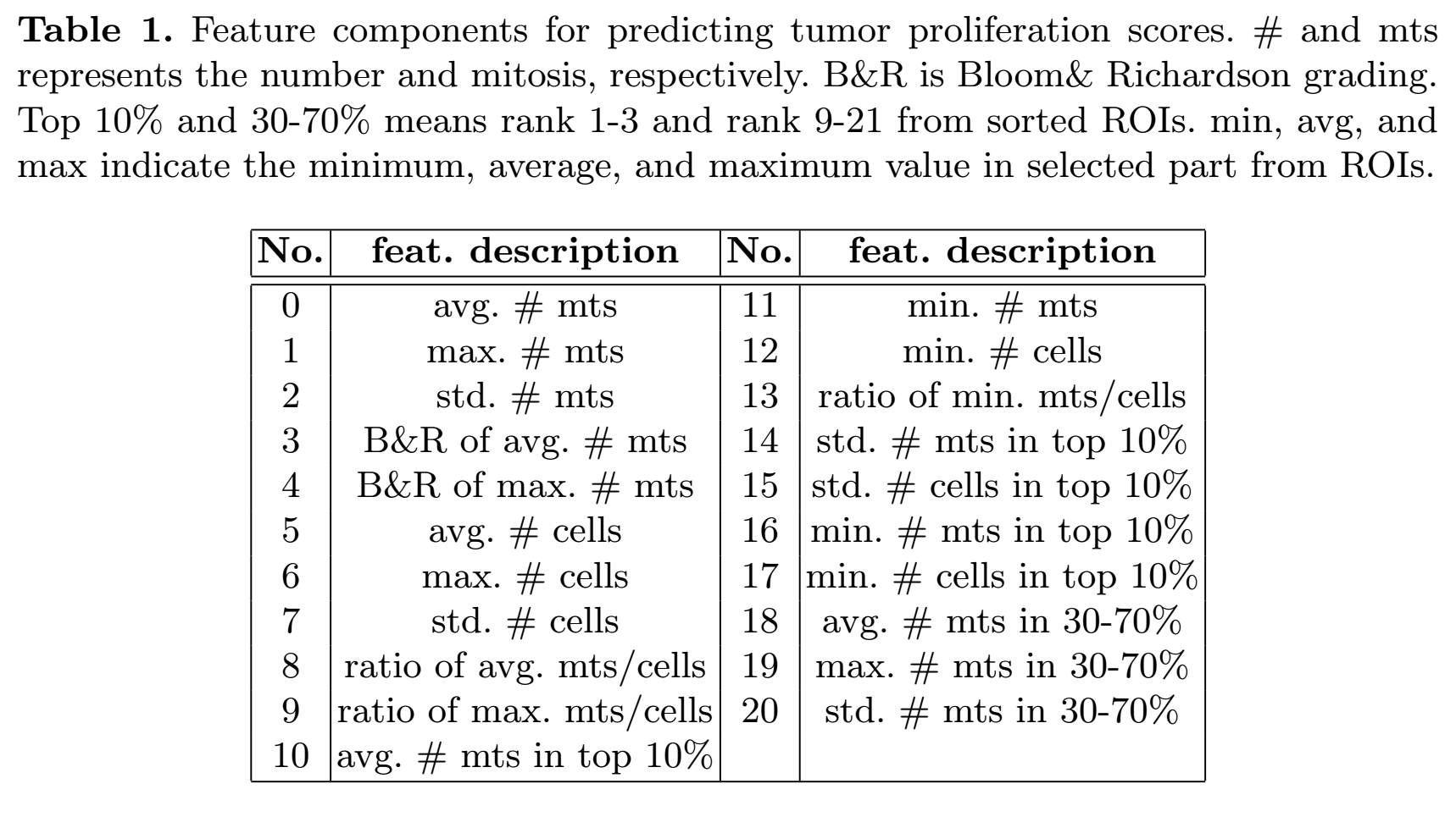
3, Tumor Proliferation Score Prediction. Apated SVM model and Features to bechoosen(Fig.6):

Fig.6

总结：这篇文章中利用了有丝分裂区域图像（小尺寸，128*128）训练了一个FCN网络，去完成在大尺寸图片中对有丝分裂区域的 detection。并注意到了 zero-padding 的影响。