深度强化学习系列之（8）----- A3C算法原理及Tensorflow实现

在DQN、DDPG算法中均用到了一个非常重要的思想经验回放，而使用经验回放的一个重要原因就是打乱数据之间的相关性，使得强化学习的序列满足独立同分布。

本文首先从Google于ICML2016顶会上发的论文《Asynchronous Methods for Deep Reinforcement Learning》解读开始，点击查看原始论文，里面的其中一大牛作者是David Sliver(看他的课入坑的)，先放个论文照片！
这里写图片描述

从论文title中就可以看出是关于Asynchronous method的内容，而且文章开头摘要中提出了一种轻量级的异步学习框架，这种框架使用了异步梯度下降来最优化神经网络。原文是：“asynchronously execute multiple agents in parallel,” 的意思，在四中不同的算法使用了多个acotr-learner ，最终能够稳定的收敛。另外在Atar、TORCS游戏以及连续性动作空间的Mujoco上均取得不错的效果。这里面最大的功劳在于他们使用了CPU多核属性，也可以说高效率的使用了计算资源。

先说第一个问题：

DQN、DDPG算法使用的experience replay(经验重放)，可以说是解决了强化学习满足独立同分布的问题，然而有优点点的背后也是有代价的，就是它使用了更多的资源和每次交互过程的计算，并且他需要一个off-policy学习算法去更新由旧策略产生的数据(experience replay has several drawbacks: it uses more memory and computation per real interaction; and it requires off-policy learning algorithms that can update from data generated by an older policy.)

于是作者就提出了“在多个环境实例上并行地异步执行多个智能体(asynchronously execute multiple agents in parallel, on multiple instances of the environment)”的概念，它的优点在于不像传统方法使用GPU或者大规模的分布式(massively distributed architectures)进行计算，而是运行在一个“多核CPU单机”上，这为普通玩家（我）带来的更多的福利。让我们更震惊的就是处理同样的任务，异步的A3C算法(后文讲解)取得了同样甚至超越的效果，而且代价就是训练的时间更短………

至于related work部分不详述，感兴趣的请自行阅读原文。

基于值函数的无模型强化学习中，通常使用神经网络作为一个逼近器来近似值函数

Q (s, a) \approx Q (s, a, θ)

$Q(s,a) \approx Q(s,a,\theta)$
在one-step Q-learning 中，朝着 one-step return 的方向去更新 Q(s, a)。但是利用 one-step 方法的缺陷在于：得到一个奖励 r 仅仅直接影响了得到该奖励的状态动作对 (s, a) 的值（obtain a reward r only directly affects the value of the state action pairs s, a that led to the reward）。其他 state action pairs的值仅仅间接的通过更新 value Q(s, a) 来影响。这就使得学习过程缓慢(耗时的原因啊)，因为许多更新都需要传播一个 reward 给相关进行的 states 和 actions。一种快速的传播奖赏的方法是利用 n-step returns。在 n-step Q-learning 中，Q(s, a) 是朝向 n-step return 进行更新。这样就使得一个奖赏 r 直接地影响了 n 个正在进行的 state action pairs 的值。这也使得给相关 state-action pairs 的奖赏传播更加有效。在 n-step Q-learning 过程中，Q(s, a) 是朝向 n-step return 定义为：

r_{t} + γ r_{t + 1} + . . . + γ^{(n - 1)} r_{t + n - 1} + max_{a} γ^{n} Q (s_{t + n}, a)

$r_{t}+\gamma r_{t+1}+...+\gamma^{(n-1)}r_{t+n−1}+\max_{a}\gamma ^{n}Q(s_{t+n},a)$
这个结果在一次奖赏 r 直接影响了 n 个后续状态动作对（n proceding state action pairs）．这就使得传递奖赏的过程变得非常有效。对比 value-based methods, policy-based model-free methods 直接参数化策略

π (a | s; θ)

$\pi(a|s;\theta)$ 并通过执行

E [R_{t}]

$E[R_{t}]$ 梯度下降来更新参数。

通常情况标准的强化学习更新策略参数 $\theta$ 的时候通常是在其策略梯度的方向 $\nabla_{\theta}\log \pi(a_{t}|s_{t};\theta)R_{t}$ ，并且 $\nabla_{\theta}E[R_{t}]$ 是无偏估计，通过从return减去被称为基线状态 $b_{t}(s_{t}）$ 的学习函数，可以减小该估计的方差，同时保持其无偏。得到的梯度是 $\nabla_{\theta}\log \pi(a_{t}|s_{t};\theta)(R_{t}-b_{t})$ 。

第二个问题

此时，我们可以定义一个新的 function A(s, a) ，这个函数称为 优势函数（advantage function）:

A (s_{t}, a_{t}) = Q (s_{t}, a_{t}) - V (s_{t})

$A(s_{t},a_{t})= Q(s_{t},a_{t})-V(s_{t})$
注意： 值函数的学习估计通常用作基线

b_{t} (s_{t} ） \approx V_{π} （ s_{t}

$b_{t}(s _{t}）≈V_{\pi}（s_{t}$ ，导致政策梯度的方差估计低得多。当使用近似值函数作为基线时，用于缩放政策梯度的数量

（ R_{t} - b_{t} ）

$（R_{t}-b_{t}）$ 可以被看作是对状态

s_{t}

$s_{t}$ 的行动的优势的估计，

R_{t}

$R_{t}$ 是

Q_{π} (s_{t}, a_{t})

$Q_{\pi}(s_{t},a_{t})$ 的估计值，

b_{t}

$b_{t}$ 是

V_{π} (s_{t})

$V_{\pi}(s_{t})$ 的估计值。

这里的优势其实也可以这么理解，对于值函数和动作值函数树来说，
这里写图片描述
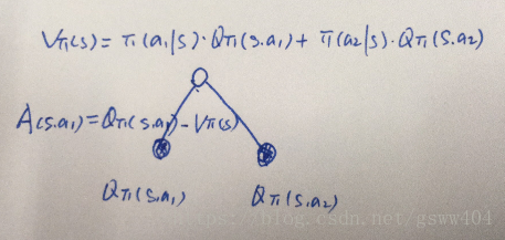
其中的 $v_{\pi}$ 可以理解为在该状态s下所有可能动作对应的动作值函数乘采取该动作的概率的和，通俗的说，值函数 $V(s)$ 是该状态下所有动作值函数关于动作概率的期望，而动作值函数 $Q(s,a)$ 是单个动作所对应的值函数，因此 $Q(s_{t},a_{t})-V(s_{t})$ 能评价当前动作值函数相对于平均值的大小。

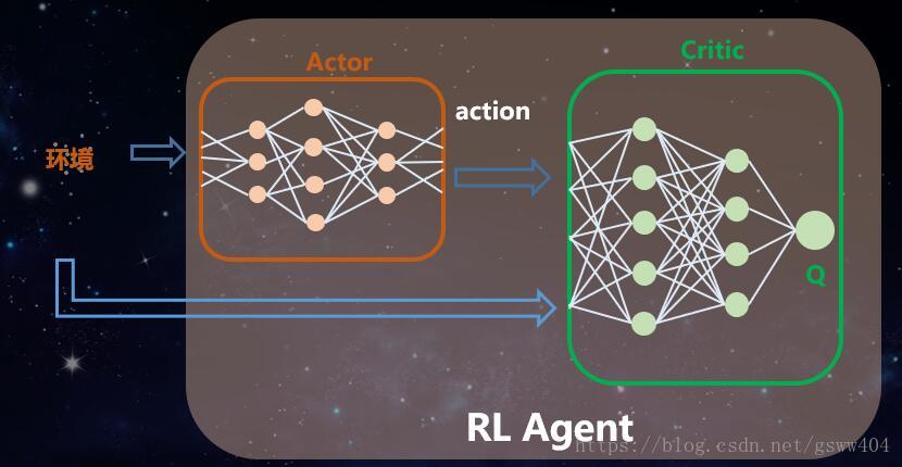
这种方法可以被视为一种行为者 - 批评者的架构”,框架结构如下，他们共同组成了强化学习的智能体：

这里写图片描述

接下来论文中讲述了Q_Learning等一系列方法，并在离散型、连续性控制任务中进行了测试，但是本文重点讲述A3C算法，为什么呢？

因为A3C既可以解决离散型控制，也可以进行连续性动作空间的控制
继续回到前面图片。因此目标就是找到一个优秀的策略，为了得到更好的 policy，我们必须进行训练更新。那么，如何来优化这个问题呢？我们需要某些度量来衡量的好坏。我们定义一个函数 $J(\pi)$ ，表示一个策略所能得到的折扣的奖赏，从初始状态 $S_{0}$ 出发得到的所有的平均：

J (π) = E_{ρ^{s_{0}}} [V (s_{0})]

$J(\pi) = E_{\rho^{s_{0}}}[V(s_{0})]$
我们发现这个函数的确很好的表达了一个 policy 有多好。但是问题是很难估计，我们需要关注的仅仅是如何改善其质量就行了。如果我们知道这个 function 的 gradient，就变的很 trivial

梯度的推到过程见 Policy Gradient 的原始paper：Policy Gradient Methods for Reinforcement Learning with Function Approximation
或者是 David Silver 的 YouTube 课程：https://www.youtube.com/watch?v=KHZVXao4qXs

而策略梯度公式可以表示为：

\nabla_{θ} J = E_{s \sim ρ^{s_{0}}, a \sim π (s)} [A (s, a) \cdot \nabla_{θ} \log π (a | s)]

$\nabla_{\theta} J = E_{s \sim \rho^{s_{0}}, a \sim \pi(s)}[A(s,a) \cdot \nabla_{\theta}\log \pi(a|s)]$
简单而言，这个期望内部的两项：

第一项，是优势函数，选择该 action 的优势，当低于 average value 的时候，该项为 negative，当比 average 要好的时候，该项为 positive；是一个标量（scalar）
第二项，告诉我们了使得 log 函数增加的方向；

到这里，所有的问题就在actor-critic框架上，即对policy梯度和值函数的更新，那么我们首先要计算的是优势函数 $A(s,a)$ 将其展开：

A (s, a) = Q (s, a) - V (s) = r + γ V (s^{^{'}}) - V (s)

$A(s,a) = Q(s,a)-V(s) = r+\gamma V(s^{'})-V(s)$
运行一次得到的 sample 可以给我们提供一个

Q (s, a)

$Q(s, a)$ 函数的 unbiased estimation。我们知道，这个时候，我们仅仅需要知道 V(s) 就可以计算 A(s, a）。这个 value function 是容易用神经网络来计算的，就像在 DQN 中估计 action-value function 一样。相比较而言，这个更简单，因为每个 state 仅仅有一个 value。

可以总结为：　
actor：优化这个 policy，使得其表现的越来越好；
critic：尝试估计 value function，使其更加准确；

好了到这里，基本上已经把Asynchronous advantage actor-critic中的advantage actor-critic说完了，最后就是到底怎么Asynchronous （异步）的呢？

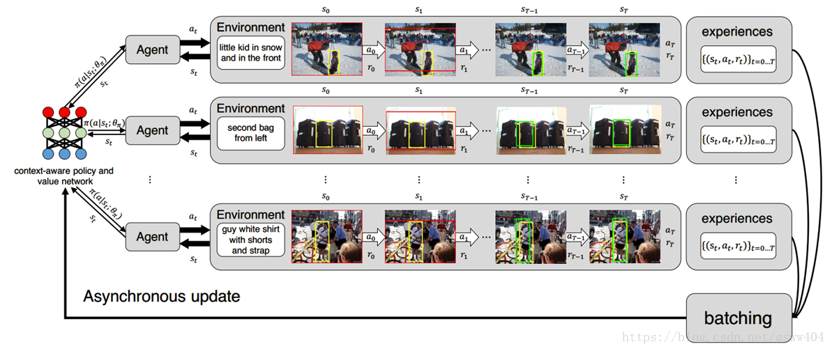
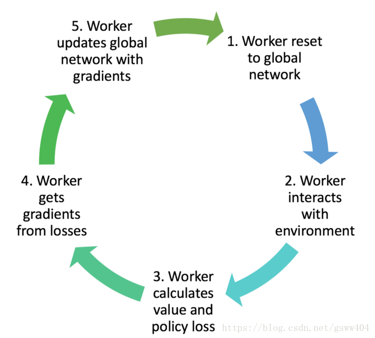
用一句话概括一下：训练的时候，同时为多个线程上分配task，学习一遍后，每个线程将自己学习到的参数更新（这里就是异步的思想）到全局Global Network上，下一次学习的时候拉取全局参数，继续学习。网络结构如图：

这里写图片描述

思考：每个异步更新是否能够使得全局网络的梯度逐渐下降呢？

上图更加形象具体点的表示就是这样的图：
这里写图片描述
而算法的执行流程是：

具体的算法伪代码如下：
这里写图片描述

本文以gym：Pendulum-v0 环境为例子，因为相对于一个状体，三个连续动作空间的摆干例子来说相对与容易解释。
tensorflow代码如下

import multiprocessing
import threading
import tensorflow as tf
import numpy as np
import gym
import os
import shutil
import matplotlib.pyplot as plt

GAME = 'Pendulum-v0'
OUTPUT_GRAPH = True
LOG_DIR = './log'
N_WORKERS = multiprocessing.cpu_count()
MAX_EP_STEP = 200
MAX_GLOBAL_EP = 2000
GLOBAL_NET_SCOPE = 'Global_Net'
UPDATE_GLOBAL_ITER = 10
GAMMA = 0.9
ENTROPY_BETA = 0.01
LR_A = 0.0001    # learning rate for actor
LR_C = 0.001    # learning rate for critic
GLOBAL_RUNNING_R = []
GLOBAL_EP = 0

env = gym.make(GAME)

# 获取状态，动作空间
N_S = env.observation_space.shape[0]
N_A = env.action_space.shape[0]
A_BOUND = [env.action_space.low, env.action_space.high]


class ACNet(object):
    def __init__(self, scope, globalAC=None):

        if scope == GLOBAL_NET_SCOPE:   # get global network
            with tf.variable_scope(scope):
                self.s = tf.placeholder(tf.float32, [None, N_S], 'S')
                self.a_params, self.c_params = self._build_net(scope)[-2:]
        else:   # local net, calculate losses
            with tf.variable_scope(scope):
                self.s = tf.placeholder(tf.float32, [None, N_S], 'S')
                self.a_his = tf.placeholder(tf.float32, [None, N_A], 'A')
                self.v_target = tf.placeholder(tf.float32, [None, 1], 'Vtarget')

                mu, sigma, self.v, self.a_params, self.c_params = self._build_net(scope)

                td = tf.subtract(self.v_target, self.v, name='TD_error')
                with tf.name_scope('c_loss'):
                    self.c_loss = tf.reduce_mean(tf.square(td))

                with tf.name_scope('wrap_a_out'):
                    mu, sigma = mu * A_BOUND[1], sigma + 1e-4

                normal_dist = tf.distributions.Normal(mu, sigma)

                with tf.name_scope('a_loss'):
                    log_prob = normal_dist.log_prob(self.a_his)
                    exp_v = log_prob * tf.stop_gradient(td)
                    entropy = normal_dist.entropy()  # encourage exploration
                    self.exp_v = ENTROPY_BETA * entropy + exp_v
                    self.a_loss = tf.reduce_mean(-self.exp_v)

                with tf.name_scope('choose_a'):  # use local params to choose action
                    self.A = tf.clip_by_value(tf.squeeze(normal_dist.sample(1), axis=[0, 1]), A_BOUND[0], A_BOUND[1])
                with tf.name_scope('local_grad'):
                    self.a_grads = tf.gradients(self.a_loss, self.a_params)
                    self.c_grads = tf.gradients(self.c_loss, self.c_params)

            with tf.name_scope('sync'):
                with tf.name_scope('pull'):
                    self.pull_a_params_op = [l_p.assign(g_p) for l_p, g_p in zip(self.a_params, globalAC.a_params)]
                    self.pull_c_params_op = [l_p.assign(g_p) for l_p, g_p in zip(self.c_params, globalAC.c_params)]
                with tf.name_scope('push'):
                    self.update_a_op = OPT_A.apply_gradients(zip(self.a_grads, globalAC.a_params))
                    self.update_c_op = OPT_C.apply_gradients(zip(self.c_grads, globalAC.c_params))

    def _build_net(self, scope):
        w_init = tf.random_normal_initializer(0., .1)
        with tf.variable_scope('actor'):
            l_a = tf.layers.dense(self.s, 200, tf.nn.relu6, kernel_initializer=w_init, name='la')
            mu = tf.layers.dense(l_a, N_A, tf.nn.tanh, kernel_initializer=w_init, name='mu')
            sigma = tf.layers.dense(l_a, N_A, tf.nn.softplus, kernel_initializer=w_init, name='sigma')
        with tf.variable_scope('critic'):
            l_c = tf.layers.dense(self.s, 100, tf.nn.relu6, kernel_initializer=w_init, name='lc')
            v = tf.layers.dense(l_c, 1, kernel_initializer=w_init, name='v')  # state value
        a_params = tf.get_collection(tf.GraphKeys.TRAINABLE_VARIABLES, scope=scope + '/actor')
        c_params = tf.get_collection(tf.GraphKeys.TRAINABLE_VARIABLES, scope=scope + '/critic')
        return mu, sigma, v, a_params, c_params

    def update_global(self, feed_dict):  # run by a local
        SESS.run([self.update_a_op, self.update_c_op], feed_dict)  # local grads applies to global net

    def pull_global(self):  # run by a local
        SESS.run([self.pull_a_params_op, self.pull_c_params_op])

    def choose_action(self, s):  # run by a local
        s = s[np.newaxis, :]
        return SESS.run(self.A, {self.s: s})


class Worker(object):
    def __init__(self, name, globalAC):
        self.env = gym.make(GAME).unwrapped
        self.name = name
        self.AC = ACNet(name, globalAC)

    def work(self):
        global GLOBAL_RUNNING_R, GLOBAL_EP
        total_step = 1
        buffer_s, buffer_a, buffer_r = [], [], []
        while not COORD.should_stop() and GLOBAL_EP < MAX_GLOBAL_EP:
            s = self.env.reset()
            ep_r = 0
            for ep_t in range(MAX_EP_STEP):
                # if self.name == 'W_0':
                #     self.env.render()
                a = self.AC.choose_action(s)
                s_, r, done, info = self.env.step(a)
                done = True if ep_t == MAX_EP_STEP - 1 else False

                ep_r += r
                buffer_s.append(s)
                buffer_a.append(a)
                buffer_r.append((r+8)/8)    # normalize

                if total_step % UPDATE_GLOBAL_ITER == 0 or done:   # update global and assign to local net
                    if done:
                        v_s_ = 0   # terminal
                    else:
                        v_s_ = SESS.run(self.AC.v, {self.AC.s: s_[np.newaxis, :]})[0, 0]
                    buffer_v_target = []
                    for r in buffer_r[::-1]:    # reverse buffer r
                        v_s_ = r + GAMMA * v_s_
                        buffer_v_target.append(v_s_)
                    buffer_v_target.reverse()

                    buffer_s, buffer_a, buffer_v_target = np.vstack(buffer_s), np.vstack(buffer_a), np.vstack(buffer_v_target)
                    feed_dict = {
                        self.AC.s: buffer_s,
                        self.AC.a_his: buffer_a,
                        self.AC.v_target: buffer_v_target,
                    }
                    self.AC.update_global(feed_dict)
                    buffer_s, buffer_a, buffer_r = [], [], []
                    self.AC.pull_global()

                s = s_
                total_step += 1
                if done:
                    if len(GLOBAL_RUNNING_R) == 0:  # record running episode reward
                        GLOBAL_RUNNING_R.append(ep_r)
                    else:
                        GLOBAL_RUNNING_R.append(0.9 * GLOBAL_RUNNING_R[-1] + 0.1 * ep_r)
                    print(
                        self.name,
                        "Ep:", GLOBAL_EP,
                        "| Ep_r: %i" % GLOBAL_RUNNING_R[-1],
                          )
                    GLOBAL_EP += 1
                    break

if __name__ == "__main__":
    SESS = tf.Session()

    with tf.device("/cpu:0"):
        OPT_A = tf.train.RMSPropOptimizer(LR_A, name='RMSPropA')
        OPT_C = tf.train.RMSPropOptimizer(LR_C, name='RMSPropC')
        GLOBAL_AC = ACNet(GLOBAL_NET_SCOPE)  # we only need its params
        workers = []
        # Create worker
        for i in range(N_WORKERS):
            i_name = 'W_%i' % i   # worker name
            workers.append(Worker(i_name, GLOBAL_AC))

    COORD = tf.train.Coordinator()
    SESS.run(tf.global_variables_initializer())

    if OUTPUT_GRAPH:
        if os.path.exists(LOG_DIR):
            shutil.rmtree(LOG_DIR)
        tf.summary.FileWriter(LOG_DIR, SESS.graph)

    worker_threads = []
    for worker in workers:
        job = lambda: worker.work()
        t = threading.Thread(target=job)
        t.start()
        worker_threads.append(t)
    COORD.join(worker_threads)

    plt.plot(np.arange(len(GLOBAL_RUNNING_R)), GLOBAL_RUNNING_R)
    plt.xlabel('step')
    plt.ylabel('Total moving reward')
    plt.show()

以上就是论文的部分和A3C算法原理及代码实现，

另外至于原始论文的实验参数、过程，后续持续补充…………………..

源码github：点击查看源代码地址

本文参考了很多资料，在这里特别特别感谢，并感谢使用莫凡的代码例子。

参考文献：
[1].Asynchronous Methods for Deep Reinforcement Learning(paper)
[2].https://www.cnblogs.com/wangxiaocvpr/p/5681483.html
[3].https://www.cnblogs.com/wangxiaocvpr/p/8110120.html
[4].https://medium.com/emergent-future/simple-reinforcement-learning-with-tensorflow-part-8-asynchronous-actor-critic-agents-a3c-c88f72a5e9f2
[5].https://github.com/MorvanZhou/Reinforcement-learning-with-tensorflow/blob/master/contents/10_A3C/A3C_continuous_action.py