Deep Learning 基础 -- 混淆矩阵、准确率、召回率、F1-Score

Deep Learning 基础 – 混淆矩阵、准确率、召回率、F1-Score

Tags： Deep_Learning

---

本文主要包含如下内容：

---

混淆矩阵、准确率、召回率、F1-Score

---

混淆矩阵

---

真实情况		预测结果
	正例	反例
正例	TP（真正例）	FN（假反例）
反例	FP（假正例）	TN（真反例）

  TP：真阳（真正例），指被分类器正确分类的正例数据
  TN：真阴（真反例），指被分类器正确分类的负例数据
  FP：假阳（假正例），被错误地标记为正例数据的负例数据
  FN：假阴（假反例），被错误地标记为负例数据的正例数据
  显然：TP+FP+TN+FN = 样本总数

---

准确率、召回率

---

  accuracy = (TP+TN)/TP+FP+TN+FN

  查准率 = 精度 = precision = TP/(TP+FP) : 模型预测为正类的样本中，真正为正类的样本所占的比例
  查全率 = 召回率 = recall = TP/(TP+FN) : 模型正确预测为正类的样本的数量，占总的正类样本数量的比值
  一般来说，查准率高时，查全率往往偏低；查全率高时，查准率往往偏低。

---

P-R曲线、F1-Score

---

  P-R曲线：查准率-查全率曲线：precision为纵轴，recall为横轴
  
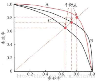
  根据P-R曲线的性能度量方式：

    第一种：    若学习器的P-R曲线被另一个学习器完全“包住”，则后者的性能优于前者；
    第二种：    若两个学习器的P-R曲线发生了交叉，可以运用平衡点（Break-Even Point，BEP），即根据在“查准率=查全率”时的取值，判断学习器性能的好坏。
    第三种：    若两个学习器的P-R曲线发生了交叉，亦可以使用F1/F_\beta度量，分别表示查准率和查全率的调和平均和加权调和平均。其中，F2分数中，召回率的权重高于准确率，而F0.5分数中，准确率的权重高于召回率。 F_\beta的物理意义就是将准确率和召回率这两个分值合并为一个分值，在合并的过程中，召回率的权重是准确率的\beta倍。F1分数认为召回率和准确率同等重要，F2分数认为召回率的重要程度是准确率的2倍，而F0.5分数认为召回率的重要程度是准确率的一半。
    第四种:     若两个学习器的P-R曲线发生了交叉，亦可以使用AP\MAP：即计算P-R曲线下的面积

$$\frac{1}{F_1} = \frac{1}{2}\times(\frac{1}{precison}+\frac{1}{recall})$$

$$F_1 = \frac {2\times precison\times recall} { precison+ recall}$$

$$\frac{1}{F_\beta} = \frac{1}{(\beta^2+1)}\times(\frac{1}{precison}+\frac{\beta^2}{recall})$$

$$F_\beta = \frac {(\beta^2+1)\times precison\times recall} {\beta^2 \times precison+ recall}$$

	准确率	召回率
A	80%	90%
B	90%	80%

  在上述表格的情况下，A/B的F1-Score是一样，因此，考虑$F_\beta-Score$加以区分，根据实际情况，选择准确率比重大还是召回率比重大。

---

AP、MAP

---

  AP（Average Precision），即平均精确度， P-R曲线下的面积 ：记 $recall = R$，$precision=P(R)$, 则 $AP=\int^1_0P(R)dR$, 实际采用：其中，M为测试集中正样本的数量

$$AP =\frac{1}{M} \sum_{m=1}^MP(\frac{m}{M})$$

  MAP：各类AP的算术平均，所有结果排序的AP平均

  检测与分类：绘制PR曲线时，分类任务取不同的score置信度阈值（confidencethresholds），检测任务取不同的IOU阈值

---

TPR、FPR、TNR

---

  真正例率 = true positive rate = sensitivity = TPR = TP/(TP+FN) ： 同recall

  假正例率 = false positive rate = FPR = FP/(FP+TN) ： 模型错分为正类的负样本，占总的负样本数量的比值

  真负类率 = rue Negative Rate = specificity = TNR = 1 - FPR

---

ROC、AUC

---

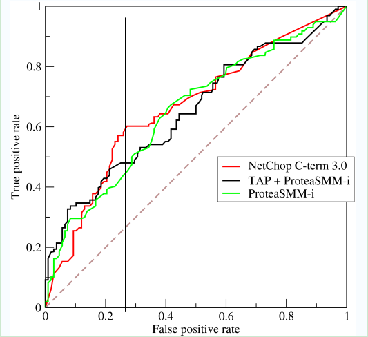
  ROC曲线，全称是受试者工作特征（Recevier Operating Characteristic）：以TPR为纵轴，FPR为横轴。
  使用情况：在类别严重不平衡的情况下（现实中样本在不同类别上的不均衡分布(class distribution imbalance problem)）,Precision和Recall无法准确刻画模型性能，此时P-R曲线度量没有意义。如正样本99个,负样本1个,直接把所有样本分类为正样本,识别率即可达到99%。此时引入ROC曲线，一般希望TPR较高，FPR较低。
  对某个分类器而言，我们可以根据模型在测试样本上的表现得到TPR和FPR点对，调整分类器分类时使用的阈值，可以得到一个经过（0,0）、（1,1）的曲线，这就是ROC曲线。 其中，将(0, 0)和(1, 1)连线形成的ROC曲线实际上代表的是一个随机分类器。
  
  根据ROC曲线的性能度量方式：

    第一种：    若学习器的ROC曲线被另一个学习器完全“包住”，则后者的性能优于前者；
    第二种：    若两个学习器的ROC曲线发生了交叉，可以计算ROC曲线下的面积，即AUC(Area Under ROC Curve)。

  AUC(Area Under ROC Curve)：ROC曲线下的面积；其中，1为完美分类器，0.5为随机猜测
  AUC值的定义：

AUC值为ROC曲线所覆盖的区域面积，显然，AUC越大，分类器分类效果越好。
AUC = 1，是完美分类器，采用这个预测模型时，不管设定什么阈值都能得出完美预测。绝大多数预测的场合，不存在完美分类器。
0.5 < AUC < 1，优于随机猜测。这个分类器（模型）妥善设定阈值的话，能有预测价值。
AUC = 0.5，跟随机猜测一样（例：丢铜板），模型没有预测价值。
AUC < 0.5，比随机猜测还差；但只要总是反预测而行，就优于随机猜测。

  AUC值的物理意义：假设分类器的输出是样本属于正类的socre（置信度），则AUC的物理意义为，任取一对（正、负）样本，正样本的score大于负样本的score的概率 (score指样本属于正例的概率)

---

新写python层计算混淆矩阵

---

  编写相应的 python layer，在caffe中调用该层，即可得到相应的输出，得到想要的混淆矩阵计算结果。

import caffe
import json
import numpy as np
import sys

import sklearn.metrics

class PythonConfMat(caffe.Layer):
    """
    Compute the ConfMat with a Python Layer
    """

    def setup(self, bottom, top):
        # check input pair
        if len(bottom) != 2:    # 检查输入 bottom 是否有两个
            raise Exception("Need two inputs to compute ConfMat.")

        self.num_labels = bottom[0].channels    # 获得 bottom[0] 的通道数
        params = json.loads(self.param_str)
        self.test_iter = params['test_iter']    # 获得测试集的迭代次数（这里使用 json.loads ）
        self.conf_matrix = np.zeros((self.num_labels, self.num_labels))     # 定义混淆矩阵，维度为分类类别
        self.current_iter = 0   # 当前迭代次数

    def reshape(self, bottom, top):
        # bottom[0] are the net's outputs
        # bottom[1] are the ground truth labels
        # Net outputs and labels must have the same number of elements
        if bottom[0].num != bottom[1].num:
            raise Exception("Inputs must have the same number of elements.")
        # accuracy output is scalar
        top[0].reshape(1)   # 输出准确率，对应一个输出

    def forward(self, bottom, top):     # 前向传播
        self.current_iter += 1      # 当前迭代次数 +1

        # predicted outputs
        pred = np.argmax(bottom[0].data, axis=1)    # 预测输出，获取预测类别的标签
        accuracy = np.sum(pred == bottom[1].data).astype(np.float32) / bottom[0].num    # 计算准确率（对应batch）
        top[0].data[...] = accuracy

        # compute confusion matrix
        self.conf_matrix += sklearn.metrics.confusion_matrix(bottom[1].data, pred, labels=range(self.num_labels))  # 混淆矩阵对应位置 +1 

        if self.current_iter == self.test_iter:     # 打印输出
            self.current_iter = 0
            sys.stdout.write('\nCAUTION!! test_iter = %i. Make sure this is the correct value' % self.test_iter)
            sys.stdout.write('\n"param_str: \'{"test_iter":%i}\'" has been set in the definition of the PythonLayer' % self.test_iter)
            sys.stdout.write('\n\nConfusion Matrix')
            sys.stdout.write('\t'*(self.num_labels-2)+'| Accuracy')
            sys.stdout.write('\n'+'-'*8*(self.num_labels+1))
            sys.stdout.write('\n')
            for i in range(len(self.conf_matrix)):
                for j in range(len(self.conf_matrix[i])):
                    sys.stdout.write(str(self.conf_matrix[i][j].astype(np.int))+'\t')
                sys.stdout.write('| %3.2f %%' % (self.conf_matrix[i][i]*100 / self.conf_matrix[i].sum()))
                sys.stdout.write('\n')
            sys.stdout.write('Number of test samples: %i \n\n' % self.conf_matrix.sum())
            # reset conf_matrix for next test phase
            self.conf_matrix = np.zeros((self.num_labels, self.num_labels))

    def backward(self, top, propagate_down, bottom):    # 不需要定义反向传播
        pass