OpenCV3之——离散傅里叶变换DFT实例

离散傅里叶变换步骤：

第一步：将图像扩大到合适的尺寸

离散傅里叶变换的运行速度跟图片尺寸有很大关系，当图片面积为 2、3、5 的倍数时 DFT 执行效率最快，因此为了达到 DFT 的执行效率最快，经常通过添凑新的边缘像素来获取最大图像尺寸。

• 计算需要扩展的行数和列数
  OpenCV 为我们提供了这样一个函数 int getOptimalDFTSize(int vecsize)，这个函数传入一个原矩阵的行数或列数，返回最优的行数或列数。
  示例

    //将输入的图像扩展到最佳尺寸，边界用0扩充
	int m = getOptimalDFTSize(srcImage.rows);
	int n = getOptimalDFTSize(srcImage.cols);

• 扩展面积至最优
  这一步，我们可以通过 OpenCV 为我们提供的 copyMakeBorder 函数进行扩展。
  示例

//将添加的图像初始化为0
Mat padded;//添充过的图像
copyMakeBorder(srcImage, padded, 0, m - srcImage.rows, 0, n - srcImage.cols, BORDER_CONSTANT, Scalar::all(0));

函数原型

void copyMakeBorder(InputArray src, OutputArray dst,
                                 int top, int bottom, int left, int right,
                                 int borderType, const Scalar& value = Scalar() );

参数	意义
InputArray src	输入矩阵
OutputArray dst	扩展之后的矩阵
int top	顶部扩展行数
int bottom	下部扩展行数
int left	左侧扩展列数
int right	右侧扩展列数
int borderType	扩展的边界类型 BORDER_CONSTANT （ iiiiii [ abcdefgh ] iiiiiii 以指定的 i 值进行扩展 ） BORDER_REPLICATE（ aaaaaa [ abcdefgh ] hhhhhhh ） BORDER_REFLECT（ fedcba [ abcdefgh ] hgfedcb ） BORDER_WRAP（ cdefgh [ abcdefgh ] abcdefg ） BORDER_REFLECT_101（ gfedcb [ abcdefgh ] gfedcba ） BORDER_TRANSPARENT （ uvwxyz [ absdefgh ] ijklmno ）
const Scalar& value	指定的填充值

第二步：将单通道扩展至双通道，以接收 DFT 的复数结果

通过 之前学到的 merge 函数进行通道扩展。
示例

//为傅里叶变换的结果（实部和虚部）分配存储空间
//将planes数组组合成一个多通道的数组complexI
Mat planes[] = { Mat_<float>(padded),Mat::zeros(padded.size(),CV_32F) };
Mat complexI;
merge(planes, 2, complexI);

第三步：就地 in-place（输入作为输出）傅里叶变换

示例

//进行就地离散傅里叶变换
dft(complexI, complexI);

dft 函数详解
该函数的作用是对一维或二维数组进行正向或逆向傅里叶变换。
函数原型：

void dft(InputArray src, OutputArray dst, int flags = 0, int nonzeroRows = 0);

• 第一个参数：InputArray src，输入的矩阵
• 第二个参数：OutputArray dst，最后运算所得结果
• 第三个参数：int flags 转换标识符，默认值为 0 ，源码及释义：

enum DftFlags {
    /** performs an inverse 1D or 2D transform instead of the default forward
        transform. */
/** 译：
执行一维或二维的逆变换，
而不是默认的正向变换。 */
    DFT_INVERSE        = 1,
    /** scales the result: divide it by the number of array elements. Normally, it is
        combined with DFT_INVERSE. */
/** 译：
通过除以数组元素的数量对输出结果进行缩放，
通常会结合 DFT_INVERSE 使用 */
    DFT_SCALE          = 2,
    /** performs a forward or inverse transform of every individual row of the input
        matrix; this flag enables you to transform multiple vectors simultaneously and can be used to
        decrease the overhead (which is sometimes several times larger than the processing itself) to
        perform 3D and higher-dimensional transformations and so forth.*/
/** 译：
 对输入矩阵的每一行进行正向或逆向变换，
设定这个标识符将允许你同时对多个向量进行变换，
还可以减少三维和多维变换等操作的开销。*/
    DFT_ROWS           = 4,
    /** performs a forward transformation of 1D or 2D real array; the result,
        though being a complex array, has complex-conjugate symmetry (*CCS*, see the function
        description below for details), and such an array can be packed into a real array of the same
        size as input, which is the fastest option and which is what the function does by default;
        however, you may wish to get a full complex array (for simpler spectrum analysis, and so on) -
        pass the flag to enable the function to produce a full-size complex output array. */
/**这里需要详细解释一下，
首先我们知道的是傅里叶变换的结果矩阵是关于原点共轭对称的，
那么两个关于原点对称的点的值，实部相等，虚部相反，
所以我们可以在一个象限中只存储实部，在另一个对称象限中只存储虚部。
这样便可以将原来需要两个通道的存储的复数值压缩进只有一个通道的矩阵进行存储，
这也是该参数的意义所在。
dft 函数的默认执行方式是：
当输入阵列为单通道时，将使用单通道阵列压缩存储输出结果；
当输入阵列为双通道时，将使用双通道阵列存储输出结果；
当指定该参数之后，将使用双通道阵列存储输出结果。
*/
    DFT_COMPLEX_OUTPUT = 16,
    /** performs an inverse transformation of a 1D or 2D complex array; the
        result is normally a complex array of the same size, however, if the input array has
        conjugate-complex symmetry (for example, it is a result of forward transformation with
        DFT_COMPLEX_OUTPUT flag), the output is a real array; while the function itself does not
        check whether the input is symmetrical or not, you can pass the flag and then the function
        will assume the symmetry and produce the real output array (note that when the input is packed
        into a real array and inverse transformation is executed, the function treats the input as a
        packed complex-conjugate symmetrical array, and the output will also be a real array). */
/** 译：
对一维或二维复数阵列进行傅里叶变换的结果通常是一个复数阵列，
对一维或二维的共轭对称阵列（如正向变换生成的矩阵）进行变换时结果是一个实数阵列。
但是 dft 函数并不会判断输入矩阵是否是共轭对称的，
我们可以通过指定这个参数来让 dft 函数假定输入阵列是具有对称性的，来生成实数阵列。
（注意：当输入阵列是一个压缩过的一通道阵列，如 dft 函数的默认正向变换结果，
那么 dft 函数会将其视为具有共轭对称性，从而输出实数阵列）
*/
    DFT_REAL_OUTPUT    = 32,
    /** performs an inverse 1D or 2D transform instead of the default forward transform. */
    DCT_INVERSE        = DFT_INVERSE,
    /** performs a forward or inverse transform of every individual row of the input
        matrix. This flag enables you to transform multiple vectors simultaneously and can be used to
        decrease the overhead (which is sometimes several times larger than the processing itself) to
        perform 3D and higher-dimensional transforms and so forth.*/
    DCT_ROWS           = DFT_ROWS
};

• 第四个参数：int nonzeroRows，默认值为 0 ，当此参数设置为非零值时，dft 函数假定输入阵列只有第一个非零行有非零元素（正向变换）或输出阵列只有第一个非零行有非零元素（逆向变换）。
  这个方法在计算数组的互关联和卷积时非常有用。

第四步：将双通道复数矩阵转换为单通道幅度矩阵

• 先分解为单通道实部矩阵和虚部矩阵，通过 split 函数进行通道分离。
  示例

//将复数转换为幅值，即=> log(1+sqrt(Re(DFT(I))^2+Im(DFT(I))^2))
split(complexI, planes);//将多通道数组complexI分解成几个单通道数组,
//实部：planes[0] = Re(DFT(I)), 
//虚部：planes[1] = Im(DFT(I))

• 使用 magnitude 函数计算幅值矩阵
  示例

magnitude(planes[0], planes[1], planes[0]);//planes[0] = magnitude

函数原型

void magnitude(InputArray x, InputArray y, OutputArray magnitude);

• 第一个参数，矢量的浮点型 x 坐标矩阵
• 第二个参数，矢量的浮点型 y 坐标矩阵
• 第三个参数，输出的结果矩阵

---

以下步骤都是加强视觉效果

---

第五步：进行对数尺度缩放（logarithmic scale）

将计算得到的幅值范围大到难以在屏幕上显示，为了可以通过图像观察到幅值变化，我们需要将高值变为亮点，而低值变为暗点。所以我们需要将幅值转至对数级。
示例

//进行对数尺寸缩放(logarithmic scale)
magnitudeImage += Scalar::all(1);
log(magnitudeImage, magnitudeImage);//求自然对数

第六步：剪切和重分布幅度图象限

• 取行列为偶数

//剪切和重分布幅度图象限
//若有奇数行或技术列，进行频谱裁剪
magnitudeImage = magnitudeImage(Rect(0, 0, magnitudeImage.cols & -2, magnitudeImage.rows & -2));

• 矩阵重排列，将对角矩阵进行交换。

//重新排列傅里叶图像中的象限，使得原点为与图像中心
int cx = magnitudeImage.cols / 2;
int cy = magnitudeImage.rows / 2;
Mat q0(magnitudeImage, Rect(0, 0, cx, cy));//ROI区域的左上
Mat q1(magnitudeImage, Rect(cx, 0, cx, cy));//右上
Mat q2(magnitudeImage, Rect(0, cy, cx, cy));//左下
Mat q3(magnitudeImage, Rect(cx, cy, cx, cy));//右下

//交换象限（左上与右下进行交换）
Mat tmp;
q0.copyTo(tmp);
q3.copyTo(q0);
tmp.copyTo(q3);
//交换象限（右上与左下交换）
q1.copyTo(tmp);
q2.copyTo(q1);
tmp.copyTo(q2);

• 现在有了重分布后的幅度图，但是仍然超出了 0-1 的范围、使用 normalize 函数归一化到可显示范围

//归一化，用0到1之间的浮点值将矩阵变换为可视的图像格式
normalize(magnitudeImage, magnitudeImage, 0, 1, NORM_MINMAX);

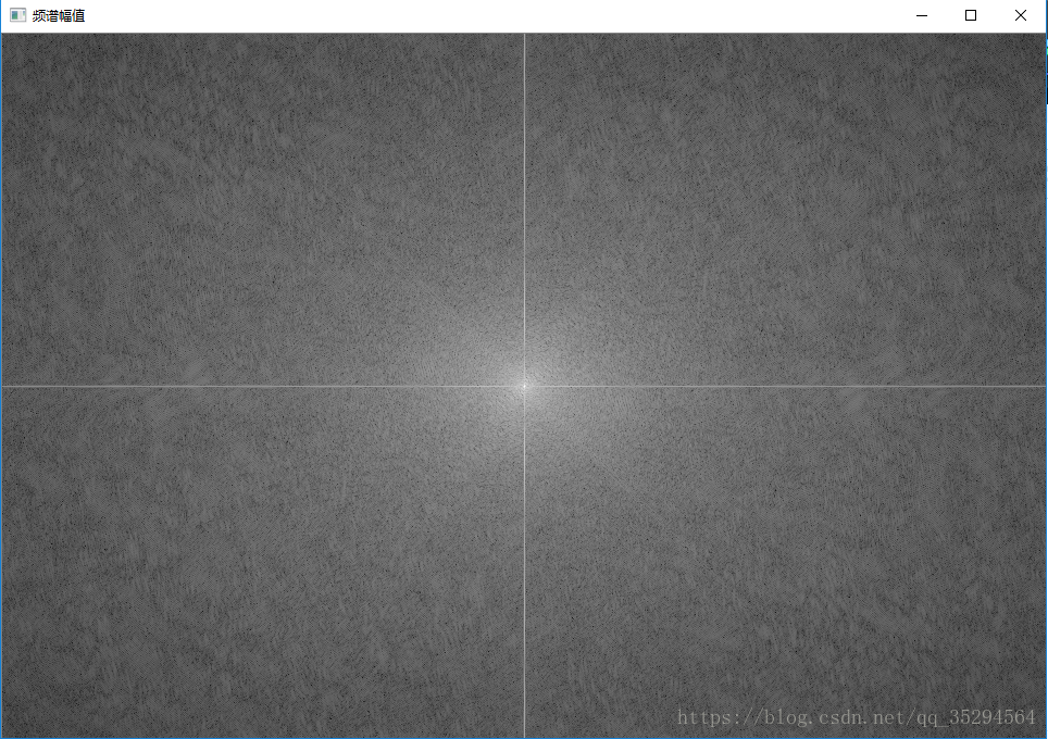
第六步：显示幅值图

//显示效果图
imshow("频谱幅值", magnitudeImage);

---

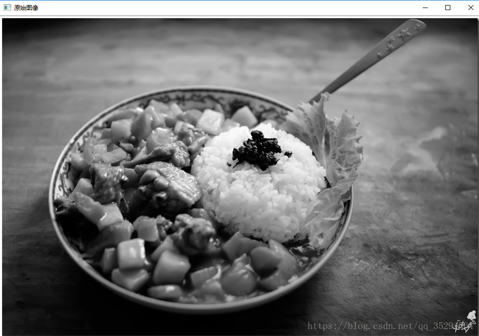
OpenCV 计算并可视化二维 DFT 结束，以下是完整代码和运行效果图。

---

完整代码

//头文件
#include <opencv2/opencv.hpp>
using namespace cv;

int main(int argc, char** argv) {
	//以灰度图模式读取原图像并显示
	Mat srcImage = imread("1.jpg", 0);
	if (!srcImage.data) {
		printf("读取图片错误！");
		return false;
	}
	imshow("原始图像", srcImage);

	//将输入的图像扩展到最佳尺寸，边界用0扩充
	int m = getOptimalDFTSize(srcImage.rows);
	int n = getOptimalDFTSize(srcImage.cols);
	//将添加的图像初始化为0
	Mat padded;//添充过的图像
	copyMakeBorder(srcImage, padded, 0, m - srcImage.rows, 0, n - srcImage.cols, BORDER_CONSTANT, Scalar::all(0));

	//为傅里叶变换的结果（实部和虚部）分配存储空间
	//将planes数组组合成一个多通道的数组complexI
	Mat planes[] = { Mat_<float>(padded),Mat::zeros(padded.size(),CV_32F) };
	Mat complexI;
	merge(planes, 2, complexI);

	//进行就地离散傅里叶变换
	dft(complexI, complexI);

	//将复数转换为幅值，即=> log(1+sqrt(Re(DFT(I))^2+Im(DFT(I))^2))
	split(complexI, planes);//将多通道数组complexI分解成几个单通道数组,
	//实部：planes[0] = Re(DFT(I)), 
	//虚部：planes[1] = Im(DFT(I))
	magnitude(planes[0], planes[1], planes[0]);//planes[0] = magnitude
	Mat magnitudeImage = planes[0];

	//进行对数尺寸缩放(logarithmic scale)
	magnitudeImage += Scalar::all(1);
	log(magnitudeImage, magnitudeImage);//求自然对数

	//剪切和重分布幅度图象限
	//若有奇数行或技术列，进行频谱裁剪
	magnitudeImage = magnitudeImage(Rect(0, 0, magnitudeImage.cols & -2, magnitudeImage.rows & -2));
	//重新排列傅里叶图像中的象限，使得原点为与图像中心
	int cx = magnitudeImage.cols / 2;
	int cy = magnitudeImage.rows / 2;
	Mat q0(magnitudeImage, Rect(0, 0, cx, cy));//ROI区域的左上
	Mat q1(magnitudeImage, Rect(cx, 0, cx, cy));//右上
	Mat q2(magnitudeImage, Rect(0, cy, cx, cy));//左下
	Mat q3(magnitudeImage, Rect(cx, cy, cx, cy));//右下

	//交换象限（左上与右下进行交换）
	Mat tmp;
	q0.copyTo(tmp);
	q3.copyTo(q0);
	tmp.copyTo(q3);
	//交换象限（右上与左下交换）
	q1.copyTo(tmp);
	q2.copyTo(q1);
	tmp.copyTo(q2);

	//归一化，用0到1之间的浮点值将矩阵变换为可视的图像格式
	normalize(magnitudeImage, magnitudeImage, 0, 1, NORM_MINMAX);

	//显示效果图
	imshow("频谱幅值", magnitudeImage);

	waitKey();
	return 0;
	

}

运行结果：