1.PCA原理
2.PCA的实现
数据集:
64维的手写数字图像
代码:
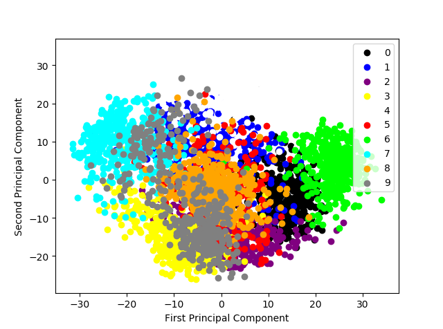
#coding=utf-8
import numpy as np
import pandas as pd
from sklearn.decomposition import PCA
from matplotlib import pyplot as plt
from sklearn.svm import LinearSVC
from sklearn.metrics import classification_report

#1.初始化一个线性矩阵并求秩
M = np.array([[1,2],[2,4]])   #初始化一个2*2的线性相关矩阵
np.linalg.matrix_rank(M,tol=None)  # 计算矩阵的秩

#2.读取训练数据与测试数据集。
digits_train = pd.read_csv('https://archive.ics.uci.edu/ml/machine-learning-databases/optdigits/optdigits.tra', header=None)
digits_test = pd.read_csv('https://archive.ics.uci.edu/ml/machine-learning-databases/optdigits/optdigits.tes', header=None)
print digits_train.shape   #(3823, 65)    3000+个样本,每个数据由64个特征,1个标签构成
print digits_test.shape    #(1797, 65)

#3将数据降维到2维并可视化

# 3.1 分割训练数据的特征向量和标记
X_digits = digits_train[np.arange(64)]         #得到64位特征值
y_digits = digits_train[64]                    #得到对应的标签

#3.2 PCA降维:降到2维
estimator = PCA(n_components=2)
X_pca=estimator.fit_transform(X_digits)

#3.3 显示这10类手写体数字图片经PCA压缩后的2维空间分布
def plot_pca_scatter():
    colors = ['black', 'blue', 'purple', 'yellow', 'white', 'red', 'lime', 'cyan', 'orange', 'gray']
    for i in xrange(len(colors)):
        px = X_pca[:, 0][y_digits.as_matrix() == i]
        py = X_pca[:, 1][y_digits.as_matrix() == i]
        plt.scatter(px, py, c=colors[i])
    plt.legend(np.arange(0, 10).astype(str))
    plt.xlabel('First Principal Component')
    plt.ylabel('Second Principal Component')
    plt.show()
plot_pca_scatter()

# 4.用SVM分别对原始空间的数据(64维)和降到20维的数据进行训练,预测

# 4.1 对训练数据/测试数据进行特征向量与分类标签的分离
X_train = digits_train[np.arange(64)]
y_train = digits_train[64]
X_test = digits_test[np.arange(64)]
y_test = digits_test[64]

#4.2 用SVM对64维数据进行进行训练
svc = LinearSVC()  # 初始化线性核的支持向量机的分类器
svc.fit(X_train,y_train)
y_pred = svc.predict(X_test)

#4.3 用SVM对20维数据进行进行训练
estimator = PCA(n_components=20)   # 使用PCA将原64维度图像压缩为20个维度
pca_X_train = estimator.fit_transform(X_train)   # 利用训练特征决定20个正交维度的方向,并转化原训练特征
pca_X_test = estimator.transform(X_test)

psc_svc = LinearSVC()
psc_svc.fit(pca_X_train,y_train)
pca_y_pred = psc_svc.predict(pca_X_test)

#5.获取结果报告
#输出用64维度训练的结果
print svc.score(X_test,y_test)
print classification_report(y_test,y_pred,target_names=np.arange(10).astype(str))

#输出用20维度训练的结果
print psc_svc.score(pca_X_test,y_test)
print classification_report(y_test,pca_y_pred,target_names=np.arange(10).astype(str))
运行结果:
1)将数据压缩到两维,在二维平面的可视化。
2)SVM对64维和20维数据的训练结果
0.9220923761825265
precision recall f1-score support
0 0.99 0.98 0.99 178
1 0.97 0.76 0.85 182
2 0.99 0.98 0.98 177
3 1.00 0.87 0.93 183
4 0.95 0.97 0.96 181
5 0.90 0.97 0.93 182
6 0.99 0.97 0.98 181
7 0.99 0.90 0.94 179
8 0.67 0.97 0.79 174
9 0.90 0.86 0.88 180
avg / total 0.94 0.92 0.92 1797
0.9248747913188647
precision recall f1-score support
0 0.97 0.96 0.96 178
1 0.88 0.90 0.89 182
2 0.96 0.99 0.97 177
3 0.99 0.91 0.95 183
4 0.92 0.96 0.94 181
5 0.87 0.96 0.91 182
6 0.98 0.97 0.98 181
7 0.98 0.89 0.93 179
8 0.91 0.83 0.86 174
9 0.83 0.88 0.85 180
avg / total 0.93 0.92 0.93 1797
结论:降维后的准确率降低,但却用了更少的维度。