本文算法完整实现源码已开源至本人的GitHub(如果对你有帮助,请给一个 star ),参看其中的 iforest 包下的 IForest 和 ITree 两个类: https://github.com/JeemyJohn/AnomalyDetection
前言
本文介绍的 Isolation Forest 算法原理请参看我的博客:Isolation Forest异常检测算法原理详解,本文中我们只介绍详细的代码实现过程。
1、ITree的设计与实现
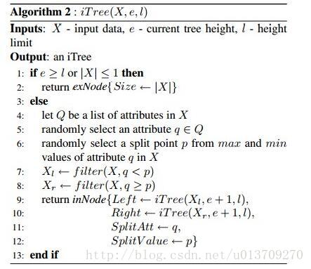
首先,我们参看原论文中的ITree的构造伪代码:
1.1 设计ITree类的数据结构
由原论文[1,2]以及上述伪代码可知,ITree是一个二叉树,并且构建ITree的算法采用的是递归构建。同时构造的结束条件是:
- 当前节点的高度超过了算法设置的阈值
l ; - 当前子树只包含一个叶节点;
- 当前子树的所有节点值的所有属性完全一致。
并且在递归的时候,我们需要随机的选择属性集
因此,我设计了如下的数据结构ITree:
public class ITree {

    // 被选中的属性索引
    public int attrIndex;

    // 被选中的属性的一个具体的值
    public double attrValue;

    // 树的总叶子节点数
    public int leafNodes;

    // 该节点在树种的高度
    public int curHeight;

    // 左右孩子书
    public ITree lTree, rTree;

    // 构造函数,初始化ITree中的值
    public ITree(int attrIndex, double attrValue) {
        // 默认高度,树的高度从0开始计算
        this.curHeight = 0;

        this.lTree = null;
        this.rTree = null;
        this.leafNodes = 1;
        this.attrIndex = attrIndex;
        this.attrValue = attrValue;
    }
   ...
}
1.2 递归地构造二叉树ITree
根据原论文中的算法2的伪代码,我们知道递归地构造二叉树ITree分为两个部分:
第一,首先判断是否满足1.1节列出的三个递归结束条件;
第二,随机的选取属性集中的一个属性以及该属性集下的一个具体的值,然后根据该属性以及生成的属性值将父节点中包含的样本数据划分到左右子树,并递归地创建左右子树。
同时记录每个节点包含的叶子节点数和当前节点在整个树中的实际高度。
参看如下的详细代码实现:
    /**
     * 根据samples样本数据递归的创建 ITree 树
     */
    public static ITree createITree(double[][] samples, int curHeight,
                                   int limitHeight)
    {

        ITree iTree = null;

        /*************** 第一步:判断递归是否满足结束条件 **************/
        if (samples.length == 0) {
            return iTree;
        } else if (curHeight >= limitHeight || samples.length == 1) {
            iTree = new ITree(0, samples[0][0]);
            iTree.leafNodes = 1;
            iTree.curHeight = curHeight;
            return iTree;
        }

        int rows = samples.length;
        int cols = samples[0].length;

        // 判断是否所有样本都一样,如果都一样构建也终止
        boolean isAllSame = true;
        break_label:
        for (int i = 0; i < rows - 1; i++) {
            for (int j = 0; j < cols; j++) {
                if (samples[i][j] != samples[i + 1][j]) {
                    isAllSame = false;
                    break break_label;
                }
            }
        }

        // 所有的样本都一样,构建终止,返回的是叶节点
        if (isAllSame == true) {
            iTree = new ITree(0, samples[0][0]);
            iTree.leafNodes = samples.length;
            iTree.curHeight = curHeight;
            return iTree;
        }


        /*********** 第二步:不满足递归结束条件,继续递归产生子树 *********/
        Random random = new Random(System.currentTimeMillis());
        int attrIndex = random.nextInt(cols);

        // 找这个被选维度的最大值和最小值
        double min, max;
        min = samples[0][attrIndex];
        max = min;
        for (int i = 1; i < rows; i++) {
            if (samples[i][attrIndex] < min) {
                min = samples[i][attrIndex];
            }
            if (samples[i][attrIndex] > max) {
                max = samples[i][attrIndex];
            }
        }

        // 计算划分属性值
        double attrValue = random.nextDouble() * (max - min) + min;

        // 将所有的样本的attrIndex对应的属性与
        // attrValue 进行比较以选出左右子树对应的样本
        int lnodes = 0, rnodes = 0;
        double curValue;
        for (int i = 0; i < rows; i++) {
            curValue = samples[i][attrIndex];
            if (curValue < attrValue) {
                lnodes++;
            } else {
                rnodes++;
            }
        }

        double[][] lSamples = new double[lnodes][cols];
        double[][] rSamples = new double[rnodes][cols];

        lnodes = 0;
        rnodes = 0;
        for (int i = 0; i < rows; i++) {
            curValue = samples[i][attrIndex];
            if (curValue < attrValue) {
                lSamples[lnodes++] = samples[i];
            } else {
                rSamples[rnodes++] = samples[i];
            }
        }

        // 创建父节点
        ITree parent = new ITree(attrIndex, attrValue);
        parent.leafNodes = rows;
        parent.curHeight = curHeight;
        parent.lTree = createITree(lSamples, curHeight + 1, limitHeight);
        parent.rTree = createITree(rSamples, curHeight + 1, limitHeight);

        return parent;
    }
2、IForest的设计与实现
原论文的算法1的伪代码如下所示:
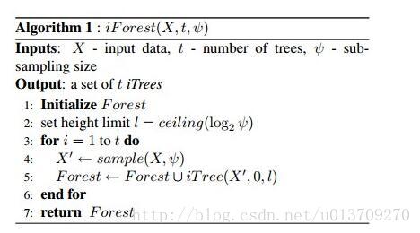
由上图的伪代码,我们知道,IForest类主要作用就是用来做两件事:
对输入数据进行子采样后构建ITree;
将所有构建的ITree合并,构成检测森林。
2.1 设计IForest类的数据结构
因此,我们设计了如下的基本数据结构类 IForest。其中
public class IForest {

    // center0代表异常类中心,center1代表正常类中心
    private Double center0;
    private Double center1;

    // 样本集子采样的数目
    private int subSampleSize;

    // IForest中包含的ITree链表
    private List<ITree> iTreeList;

    /**
     * 无参构造函数,contamination设置为默认值0.1
     */
    public IForest() {
        this.center0 = null;
        this.center1 = null;
        this.subSampleSize = 256;
        this.iTreeList = new ArrayList<>();
    }
    ...
}
2.2 构建森林
初始化玩IForest之后的第一件事,当然是构建一颗一颗的ITree,并将它们添加到
    /**
     * 创建IForest
     */
    private void createIForest(double[][] samples, int t) throws Exception {

        // 方法参数合法性检验
        if (samples == null || samples.length == 0) {
            throw new Exception("Samples is null or empty, please check...");
        } else if (t <= 0) {
            throw new Exception("Number of subtree t must be a positive...");
        } else if (subSampleSize <= 0) {
            throw new Exception("subSampleSize must be a positive...");
        }

        // 设置每颗 ITree 的高度上限
        int limitHeight = (int) Math.ceil(Math.log(subSampleSize) / Math.log(2));

        ITree iTree;
        double[][] subSample;

        for (int i = 0; i < t; i++) {
            subSample = this.getSubSamples(samples, subSampleSize);
            iTree = ITree.createITree(subSample, 0, limitHeight);
            this.iTreeList.add(iTree);
        }
    }
2.3 计算样本的异常指数
IForest构建好了之后我们就可以对每一个样本计算他们的异常指数了,异常指数的计算方法请参看我的另一篇博文,结合代码就知道了。
在这里,我们就能看出来,我们计算的
/**
* 计算某一个样本的异常指数
*/
private double computeAnomalyIndex(double[] sample) throws Exception {
if (iTreeList == null || iTreeList.size() == 0) {
throw new Exception("iTreeList is empty,please create IForest...");
} else if (sample == null || sample.length == 0) {
throw new Exception("Sample is null or empty, please check...");
}
// 样本在所有iTree上的平均高度(改进后的)
double ehx = 0;
double pathLength = 0;
for (ITree iTree : iTreeList) {
pathLength = computePathLength(sample, iTree);
ehx += pathLength;
}
ehx /= iTreeList.size();
double cn = computeCn(subSampleSize);
double index = ehx / cn;
double anomalyIndex = Math.pow(2, -index);
return anomalyIndex;
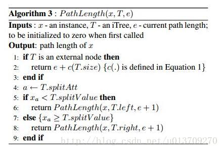
}2.4 计算路径高度
路径高度计算函数用于“估算” (为什么是估算请看上一篇博文或者原论文) 样本点在当前ITree上的高度。
/**
  * 计算样本sample在ITree上的PathLength
  */
private double computePathLength(double[] sample, final ITree iTree) throws Exception {

        // 参数合法性检查
        if (sample == null || sample.length == 0) {
            throw new Exception("Sample is null or empty, please check...");
        } else if (iTree == null || iTree.leafNodes == 0) {
            throw new Exception("iTree is null or empty, please check...");
        }

        double pathLength = -1;
        double attrValue;
        ITree tmpITree = iTree;

        while (tmpITree != null) {
            pathLength += 1;
            attrValue = sample[tmpITree.attrIndex];

            if (tmpITree.lTree == null || tmpITree.rTree == null || attrValue == tmpITree.attrValue) {
                break;
            } else if (attrValue < tmpITree.attrValue) {
                tmpITree = tmpITree.lTree;
            } else {
                tmpITree = tmpITree.rTree;
            }
        }

        return pathLength + computeCn(tmpITree.leafNodes);
    }
3、训练过程
细心的读者都会发现,上述的所有成员函数都是私有成员。这就是说无论是类还是对象都不能在主程序中调用它们,所以为了接口使用的方便一个简单的
public int[] train(double[][] samples, int t, int subSampleSize, int iters) throws Exception {

        this.subSampleSize = subSampleSize;
        if (this.subSampleSize > samples.length) {
            this.subSampleSize = samples.length;
        }

        // 第一步:创建Isolation Forest
        createIForest(samples, t);

        // 第二步:计算所有样本的异常指数
        double[] scores = computeAnomalyIndex(samples);

        // 第三步:获取类标,并设置类标中心
        int[] labels = classifyByCluster(scores, iters);
        return labels;
    }
观察训练过程,我们知道总共的训练分三步:
第一步:创建Isolation Forest;
第二步:计算所有样本的异常指数;
第三步:获取类标,并设置类标中心。
根据前面的讲解,我们能明白前两步,但是第三步我们是如何获取类标和计算类标中心的呢?原论文只讲到异常指数趋向于0就是正常样本,趋向于1就是异常样本,如果全体都趋向于0.5左右,那么全体都是正常的。
但是就这些我们也没办法去判断到底多少是异常多少是正常,怎么去找这个界限或者说阈值?
4、计算类标中心
对于计算这个阈值,我曾经想过留给用户作为算法的参数,因为不同的情况下阈值根本不一样,所以我们不能在算法中固定死它的具体取值。但是为了减少算法参数以及用户的训练次数不至于多次尝试选取阈值浪费时间的考虑,我本人灵机一动,结合KMeans聚类的思想想出了用聚类的方法计算两类异常指数的中心点。
具体的方法是这样的,因为原论文虽然没有给出如何计算和判定类标属性,但是给出了大致的方针:趋向于0就是正常样本,趋向于1就是异常样本。
根据KMeans的思想,我们首先对所有的一维数据异常指数进行KMeans计算(K=2),这样我们就能计算到两个类的类标中心。我们知道了每个类的类标中心我们不就知道每个样本是哪个类了:离哪个近就是哪个类啊!我是不是很聪明? 并且在这里,由于上述方针,我们在进行KMeans计算类中心之前可以先将直接将初始类中心点设置为所有的异常指数的最大值和最小值,这也解决了KMeans方法在选初始类中心时可能导致算法不准确的问题(想一想为什么)。 这样判断类标的问题就完美解决了。好了,看代码吧:
/**
     * 通过使用聚类的思想,根据anomalyIndex进行分类获取类标
     */
    private int[] classifyByCluster(double[] scores, int iters) {

        // 两个聚类中心
        center0 = scores[0]; // 异常类的聚类中心
        center1 = scores[0]; // 正常类的聚类中心

        // 根据原论文,异常指数接近1说明是异常点,接近0为正常点。所以,将center0、center1分别初始化为
        // scores中的最大值和最小值。这样就相当于KMeans聚类的初始点的选择,解决了KMeans聚类的不稳定性。
        for (int i = 1; i < scores.length; i++) {
            if (scores[i] > center0) {
                center0 = scores[i];
            }

            if (scores[i] < center1) {
                center1 = scores[i];
            }
        }

        int cnt0, cnt1;
        double diff0, diff1;
        int[] labels = new int[scores.length];

        // 迭代聚类(迭代iters次)
        for (int n = 0; n < iters; n++) {
            // 判断每个样本的类别
            cnt0 = 0;
            cnt1 = 0;

            for (int i = 0; i < scores.length; i++) {
                // 计算当前点与两个聚类中心的距离
                diff0 = Math.abs(scores[i] - center0);
                diff1 = Math.abs(scores[i] - center1);

                // 根据与聚类中心的距离,判断类标
                if (diff0 < diff1) {
                    labels[i] = 0;
                    cnt0++;
                } else {
                    labels[i] = 1;
                    cnt1++;
                }
            }

            // 保存旧的聚类中心
            diff0 = center0;
            diff1 = center1;

            // 重新计算聚类中心
            center0 = 0.0;
            center1 = 0.0;
            for (int i = 0; i < scores.length; i++) {
                if (labels[i] == 0) {
                    center0 += scores[i];
                } else {
                    center1 += scores[i];
                }
            }

            center0 /= cnt0;
            center1 /= cnt1;

            // 提前迭代终止条件
            if (center0 - diff0 <= 1e-6 && center1 - diff1 <= 1e-6) {
                break;
            }
        }
        return labels;
    }
5、对未知样本的预测
有了类标中心
   /**
     * 预测样本 sample 是否为异常值,正常返回1,异常返回0
     */
    public int predict(double[] sample) throws Exception {
        double score = computeAnomalyIndex(sample);
        double dis0 = Math.abs(score - center0);
        double dis1 = Math.abs(score - center1);

        // 与哪个中心近说明改点被判断为哪一类
        if (dis0 > dis1) {
            return 1;
        } else {
            return 0;
        }
    }
对机器学习,人工智能感兴趣的小伙伴,请关注我的公众号:

参考文献: