【数据异常校验】Scikit-learn实现隔离森林（Isolation Forest）算法进行异常值检测

目录

算法类

方法

实践

案例1：多种异常检测算法比较

代码

案例2

---

使用Isolation Forest算法返回每个样本的异常分数

Isolation Forest通过随机选择一个特征然后随机选择所选特征的最大值和最小值之间的分割值来“隔离”观察结果。

由于递归分区可以由树结构表示，因此隔离样本所需的分割数等于从根节点到终止节点的路径长度。

这种随机树林的平均路径长度是衡量正态性和决策函数的标准。

随机分区会产生明显较短的异常路径。因此，当随机树林共同为特定样本产生较短的路径长度时，它们很可能是异常。

在高维数据集中执行离群值检测的一种有效方法是使用随机森林。

所述ensemble.IsolationForest通过分离的观察通过随机选择一个功能，然后随机选择所选择的特征的最大值和最小值之间的分割值。

该策略如下所示。

算法类

class sklearn.ensemble.IsolationForest(n_estimators=100, max_samples=’auto’, contamination=’legacy’, max_features=1.0, bootstrap=False, n_jobs=None, behaviour=’old’, random_state=None, verbose=0)

版本0.18中的新功能。

参数:

n_estimators : int, optional (default=100) 整体中基本估算器的数量。 max_samples : int or float, optional (default=”auto”) 从X中抽取的样本数量，用于训练每个基本估算器。 如果是int，则绘制max_samples样本。 如果是float，则绘制max_samples * X.shape [0]样本。 如果是“auto”，则max_samples = min（256，n_samples）。 如果max_samples大于提供的样本数，则所有样本将用于所有树（无采样）。 contamination : float in (0., 0.5), optional (default=0.1) 数据集的污染量，即数据集中异常值的比例。在拟合时用于定义决策函数的阈值。如果是“自动”，则确定决策函数阈值，如原始论文中所示。 在版本0.20中更改：默认值contamination将从0.20更改为'auto'0.22。 max_features : int or float, optional (default=1.0) 从X中绘制以训练每个基本估计器的特征数。 如果是int，则绘制max_features特征。 如果是float，则绘制max_features * X.shape [1]特征。 bootstrap : boolean, optional (default=False) 如果为True，则单个树适合随替换采样的训练数据的随机子集。如果为假，则执行不替换的采样。 n_jobs : int or None, optional (default=None) 适合和预测并行运行的作业数。 None除非在joblib.parallel_backend上下文中，否则表示1 。 -1表示使用所有处理器。有关 详细信息，请参阅词汇表。 behaviour : str, default=’old’ 行为decision_function可以是“旧的”或“新的”。传递behaviour='new'使decision_function 更改与其他异常检测算法API相匹配，这将是未来的默认行为。如offset_属性文档中详细解释的那样，decision_function变得依赖于污染参数，使得0成为检测异常值的自然阈值。 版本0.20中的新功能：在0.20behaviour中添加，以实现后向兼容性目的。 从版本0.20开始behaviour='old'不推荐使用：在0.20中弃用，在0.22中不可能。 从版本0.22开始behaviour不推荐使用：参数将在0.22中弃用，并在0.24中删除。 random_state : int, RandomState instance or None, optional (default=None) 如果是int，则random_state是随机数生成器使用的种子; 如果是RandomState实例，则random_state是随机数生成器; 如果没有，随机数生成器所使用的RandomState实例np.random。 verbose : int, optional (default=0) 控制树构建过程的详细程度。

属性:

estimators_ : list of DecisionTreeClassifier 拟合子估算器的集合。. estimators_samples_ : list of arrays 每个基本估算器的绘制样本子集。 max_samples_ : integer 实际的样本数量 offset_ : float 偏移量用于根据原始分数定义决策函数。我们有这样的关系：。假设行为=='新'，定义如下。当污染参数设置为“自动”时，偏差等于-0.5，因为内部的分数接近0并且异常值的分数接近-1。当提供不同于“自动”的污染参数时，以这样的方式定义偏移，即我们在训练中获得预期数量的异常值（具有判定函数<0的样本）。假设行为参数设置为'old'，我们总是有 ，使决策功能独立于污染参数。decision_function = score_samples - offset_offset_offset_ = -0.5

改算法参考：

[1]	刘飞，丁婷，凯明，周志华。“隔离森林。”数据挖掘，2008年.ICDM'08。第八届IEEE国际会议。

[2]	刘飞，丁婷，凯明，周志华。“基于隔离的异常检测。”ACM数据知识发现交易（TKDD）6.1（2012）：3。

方法

decision_function(X)	基本分类器的X的平均异常分数。
fit(X[, y, sample_weight])	估算。
fit_predict(X[, y])	在X上执行异常值检测。
get_params([deep])	获取此估算工具的参数。
predict(X)	预测特定样本是否是异常值。
score_samples(X)	与原始论文中定义的异常分数相反。
set_params(**params)	设置此估算器的参数

方法详情请看：http://scikit-learn.org/stable/modules/generated/sklearn.ensemble.IsolationForest.html

实践

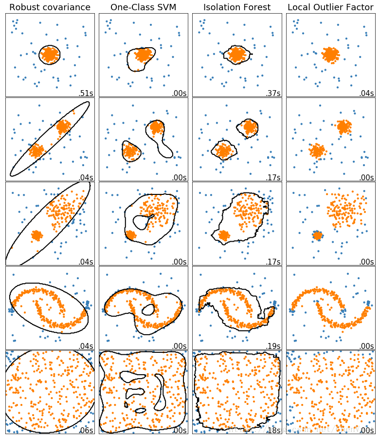
案例1：多种异常检测算法比较

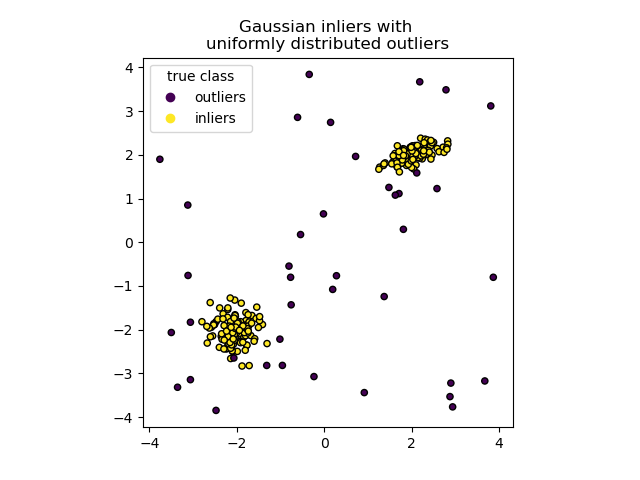
此示例显示了2D数据集上不同异常检测算法的特征。数据集包含一种或两种模式（高密度区域），以说明算法处理多模态数据的能力。

对于每个数据集，15％的样本被生成为随机均匀噪声。该比例是给予OneClassSVM的nu参数的值和其他异常值检测算法的污染参数。除了局部异常因子（LOF）之外，内部和异常值之间的决策边界以黑色显示，因为当用于异常值检测时，它没有预测方法应用于新数据。

svm.OneClassSVM被称为是对异常值敏感并因此对异常值检测不执行得非常好。当训练集未被异常值污染时，该估计器最适合于新颖性检测。也就是说，高维中的离群检测，或者对上层数据的分布没有任何假设是非常具有挑战性的，并且单类SVM可能在这些情况下根据其超参数的值给出有用的结果。

covariance.EllipticEnvelope假设数据是高斯数据并学习椭圆。因此，当数据不是单峰时，它会降级。但请注意，此估算器对异常值很稳健。

ensemble.IsolationForest并且neighbors.LocalOutlierFactor 似乎对多模态数据集表现得相当好。neighbors.LocalOutlierFactor对于第三数据集示出了优于其他估计器的优点 ，其中两种模式具有不同的密度。这一优势可以通过LOF的局部方面来解释，这意味着它只将一个样本的异常得分与其邻居的得分进行比较。

最后，对于最后一个数据集，很难说一个样本比另一个样本更异常，因为它们均匀分布在超立方体中。除了svm.OneClassSVM稍微过度拟合之外，所有估算者都为这种情况提供了不错的解决方案。在这种情况下，更仔细地观察样本的异常分数是明智的，因为良好的估计器应该为所有样本分配相似的分数。

虽然这些例子给出了一些关于算法的直觉，但这种直觉可能不适用于非常高维的数据。

最后，请注意模型的参数已经在这里精心挑选，但实际上它们需要进行调整。在没有标记数据的情况下，问题完全没有监督，因此模型选择可能是一个挑战。

代码

载入相关库

import time

import numpy as np
import matplotlib
import matplotlib.pyplot as plt

from sklearn import svm
from sklearn.datasets import make_moons, make_blobs
from sklearn.covariance import EllipticEnvelope
from sklearn.ensemble import IsolationForest
from sklearn.neighbors import LocalOutlierFactor

matplotlib.rcParams['contour.negative_linestyle'] = 'solid'

实现

# 设置
n_samples = 300
outliers_fraction = 0.15
n_outliers = int(outliers_fraction * n_samples)
n_inliers = n_samples - n_outliers

# 定义比/异常检测方法
anomaly_algorithms = [
    ("Robust covariance", EllipticEnvelope(contamination=outliers_fraction)),
    ("One-Class SVM", svm.OneClassSVM(nu=outliers_fraction, kernel="rbf",
                                      gamma=0.1)),
    ("Isolation Forest", IsolationForest(contamination=outliers_fraction,
                                         random_state=42)),
    ("Local Outlier Factor", LocalOutlierFactor(
        n_neighbors=35, contamination=outliers_fraction))]

# 定义数据集
blobs_params = dict(random_state=0, n_samples=n_inliers, n_features=2)
datasets = [
    make_blobs(centers=[[0, 0], [0, 0]], cluster_std=0.5,
               **blobs_params)[0],
    make_blobs(centers=[[2, 2], [-2, -2]], cluster_std=[0.5, 0.5],
               **blobs_params)[0],
    make_blobs(centers=[[2, 2], [-2, -2]], cluster_std=[1.5, .3],
               **blobs_params)[0],
    4. * (make_moons(n_samples=n_samples, noise=.05, random_state=0)[0] -
          np.array([0.5, 0.25])),
    14. * (np.random.RandomState(42).rand(n_samples, 2) - 0.5)]

# 在给定的设置下比较给定的分类器
xx, yy = np.meshgrid(np.linspace(-7, 7, 150),
                     np.linspace(-7, 7, 150))

plt.figure(figsize=(len(anomaly_algorithms) * 2 + 3, 12.5))
plt.subplots_adjust(left=.02, right=.98, bottom=.001, top=.96, wspace=.05,
                    hspace=.01)

plot_num = 1
rng = np.random.RandomState(42)

for i_dataset, X in enumerate(datasets):
    # 添加异常值
    X = np.concatenate([X, rng.uniform(low=-6, high=6,
                       size=(n_outliers, 2))], axis=0)

    for name, algorithm in anomaly_algorithms:
        t0 = time.time()
        algorithm.fit(X)
        t1 = time.time()
        plt.subplot(len(datasets), len(anomaly_algorithms), plot_num)
        if i_dataset == 0:
            plt.title(name, size=18)

        # 符合数据和标记异常值
        if name == "Local Outlier Factor":
            y_pred = algorithm.fit_predict(X)
        else:
            y_pred = algorithm.fit(X).predict(X)

        # 画出水平线和点
        if name != "Local Outlier Factor":  # LOF does not implement predict
            Z = algorithm.predict(np.c_[xx.ravel(), yy.ravel()])
            Z = Z.reshape(xx.shape)
            plt.contour(xx, yy, Z, levels=[0], linewidths=2, colors='black')

        colors = np.array(['#377eb8', '#ff7f00'])
        plt.scatter(X[:, 0], X[:, 1], s=10, color=colors[(y_pred + 1) // 2])

        plt.xlim(-7, 7)
        plt.ylim(-7, 7)
        plt.xticks(())
        plt.yticks(())
        plt.text(.99, .01, ('%.2fs' % (t1 - t0)).lstrip('0'),
                 transform=plt.gca().transAxes, size=15,
                 horizontalalignment='right')
        plot_num += 1

plt.show()

结果

样例详情地址： http://scikit-learn.org/stable/auto_examples/plot_anomaly_comparison.html#sphx-glr-auto-examples-plot-anomaly-comparison-py

案例2

代码

import numpy as np
import matplotlib.pyplot as plt
from sklearn.ensemble import IsolationForest

rng = np.random.RandomState(42)

# 生成训练数据
X = 0.3 * rng.randn(100, 2)
X_train = np.r_[X + 2, X - 2]
# 产生一些常规的新观察
X = 0.3 * rng.randn(20, 2)
X_test = np.r_[X + 2, X - 2]
# 产生一些异常新奇的观察结果
X_outliers = rng.uniform(low=-4, high=4, size=(20, 2))

# fit the model
clf = IsolationForest(max_samples=100,
                      random_state=rng, contamination='auto')
clf.fit(X_train)
y_pred_train = clf.predict(X_train)
y_pred_test = clf.predict(X_test)
y_pred_outliers = clf.predict(X_outliers)

# 画出直线，样本，和离平面最近的矢量
xx, yy = np.meshgrid(np.linspace(-5, 5, 50), np.linspace(-5, 5, 50))
Z = clf.decision_function(np.c_[xx.ravel(), yy.ravel()])
Z = Z.reshape(xx.shape)

plt.title("IsolationForest")
plt.contourf(xx, yy, Z, cmap=plt.cm.Blues_r)

b1 = plt.scatter(X_train[:, 0], X_train[:, 1], c='white',
                 s=20, edgecolor='k')
b2 = plt.scatter(X_test[:, 0], X_test[:, 1], c='green',
                 s=20, edgecolor='k')
c = plt.scatter(X_outliers[:, 0], X_outliers[:, 1], c='red',
                s=20, edgecolor='k')
plt.axis('tight')
plt.xlim((-5, 5))
plt.ylim((-5, 5))
plt.legend([b1, b2, c],
           ["training observations",
            "new regular observations", "new abnormal observations"],
           loc="upper left")
plt.show()

结果

样例详情地址：http://scikit-learn.org/stable/auto_examples/ensemble/plot_isolation_forest.html#sphx-glr-auto-examples-ensemble-plot-isolation-forest-py

参考&翻译：

http://scikit-learn.org/stable/modules/outlier_detection.html#isolation-forest