Tensorflow实现CNN用于MNIST识别

这篇文章一步步教如何使用tensorflow建一个CNN，并将其应用到MNIST手写体识别中，重点是了解每一步在做什么。相应的练习代码和jupyter notebook在我的github可找到。

1. 设定结构

这篇文章实现下面的一个简单的结构：

• (Input) -> [batch_size, 28, 28, 1] >> Apply 32 filter of [5x5]
• (Convolutional layer 1) -> [batch_size, 28, 28, 32]
• (ReLU 1) -> [?, 28, 28, 32]
• (Max pooling 1) -> [?, 14, 14, 32]
• (Convolutional layer 2) -> [?, 14, 14, 64]
• (ReLU 2) -> [?, 14, 14, 64]
• (Max pooling 2) -> [?, 7, 7, 64]
• [fully connected layer 3] -> [1x1024]
• [ReLU 3] -> [1x1024]
• [Drop out] -> [1x1024]

2.创建一个交互式的会话

import tensorflow as tf
sess = tf.InteractiveSession()

3. 加载MNIST数据

from tensorflow.examples.tutorials.mnist import input_data
mnist = input_data.read_data_sets('MNIST_data', one_hot = True)

4. 初始化参数

width = 28 # width of the image in pixels 
height = 28 # height of the image in pixels
flat = width * height # number of pixels in one image 
class_output = 10 # number of possible classifications for the problem

5. 创建输入输出占位符

x = tf.placeholder(tf.float32, shape = [None, flat])
y_ = tf.placeholder(tf.float32, shape = [None, class_output])

6. 将图像转为tensor

输入图像28*28像素，一个通道。 第一个维度是输入批数量的大小，可以为任意大小。第二个和第三个维度是宽和高，最后一个维度是图像的通道。

x_image = tf.reshape(x, [-1, 28, 28, 1])

7.卷积层1

定义kernal权重和偏置

这里定义一个55的核，输入通道为1；
每张图片使用32个不同kernal；
卷积层的输出为 2828*32.
kernal张量的shape为[filter_height, filter_width, in_channels, out_channels]

W_conv1 = tf.Variable(tf.truncated_normal([5, 5, 1, 32], stddev = 0.1))
b_conv1 = tf.Variable(tf.ocnstant(0.1, shape=[32])) # 32个输出需要32个偏置

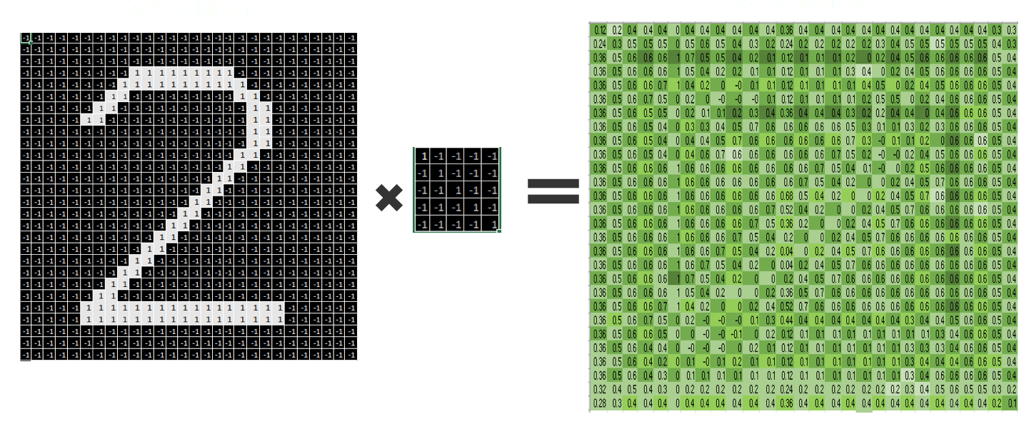
对权重做卷积并加上偏置

使用 tf.nn.conv2d创建卷积层，它用于计算给定4维输入和filter张量的2为卷积
输入：
tensor of shape [batch, in_width, in_channels], x of shape [batch_size,28 ,28, 1]
filter / kernel tensor of shape [filter_height, filter_width, in_channels, out_channels]. W is of size [5, 5, 1, 32]
stride [1, 1, 1, 1].
处理：
将filter改变为[551, 32]的2维矩阵
从输入张量中提取图像块形成一个虚拟的张量shape [batch, 28, 28, 551]
对于每一batch，右乘filter矩阵和图像向量。
输出：
一个shape为shape=(?, 28, 28, 32)的tensor，也就是32个【28*28】的图像，32是输出图像的depth。

convolve1 = tf.nn.conv2d(x_image, w_conv1, strides=[1, 1, 1, 1], padding='SAME') + b_conv1

使用ReLU激活函数

h_conv1 = tf.nn.relu(convolve1)

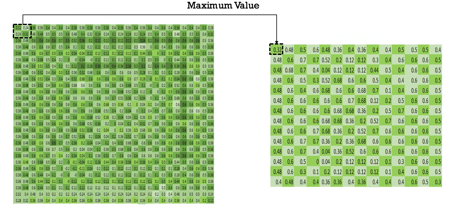
8. 最大池化

最大池化是一个非线性下采样方法，它把输入图像分成一系列的长方形，再找到每个长方形中的最大值。
使用tf.nn.max_pool函数做最大池化，Kernel size: 2x2
stride: 每次kernel滑动2个像素，没有overlapping。输入矩阵的大小为[14x14x32]，输出的大小为[14x14x32].

conv1 = tf.nn.max_pool(h_conv1, ksize=[1, 2, 2, 1], strides=[1, 2, 2, 1], padding="SAME")

输出：
<tf.Tensor ‘MaxPool:0’ shape=(?, 14, 14, 32) dtype=float32>

9. 卷积层2

kernel的权重和偏置

第二层的kernel：

• Filter/kernel: 5x5 (25 pixels)
• Input channels: 32 (from the 1st Conv layer, we had 32 feature maps)
• 64 output feature maps
  输入图像大小[14x14x32], kenel大小 [5x5x32], 使用64个核， 输出为[14x4x64]

w_conv2 = tf.Variable(tf.truncated_normal([5, 5, 32, 64], stddev=0.1))
b_conv2 = tf.Variable(tf.constant(0.1, shape=[64]))

图像与权重做卷积并加上偏置

convolve2 = tf.nn.conv2d(conv1, w_conv2, strides=[1, 1, 1, 1], padding="SAME") + b_conv2

Relu激活

h_conv2 = tf.nn.relu(convolve2)

10. 最大池化

conv2 = tf.nn.max_pool(h_conv2, ksize=[1, 2, 2, 1], strides=[1, 2, 2, 1], padding="SAME")

输出conv2为
<tf.Tensor ‘MaxPool_1:0’ shape=(?, 7, 7, 64) dtype=float32>

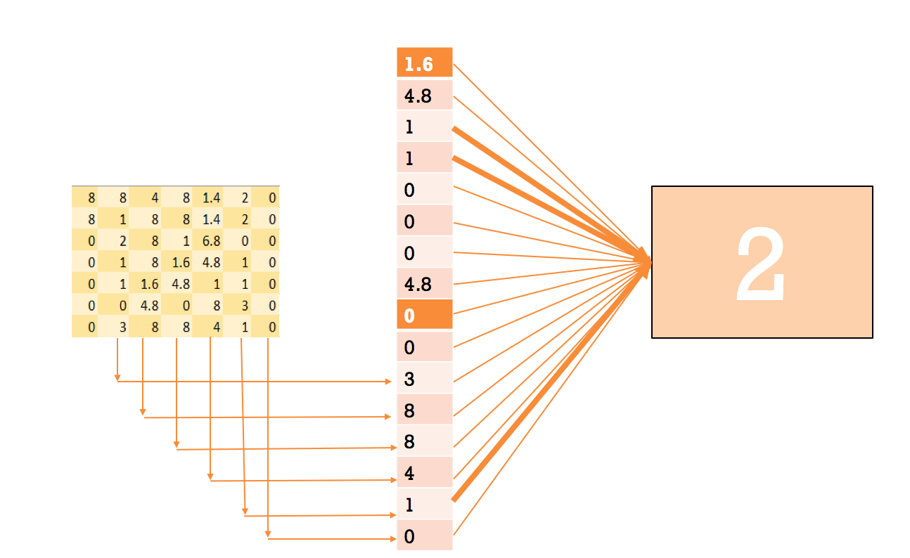
11. 全连接层

使用全连接层是为了使用softmax在最后得到概率输出。
它把前面的层中抽取深层图片，也就是最后输出的64个矩阵，展平为一列。
每一个[7x7]的矩阵会转为[49x1]的矩阵，将64个[49x1]的矩阵拼接起来得到[3136x1]的矩阵。
把它与[1024x1]的层连接起来，两层间的weight大小为[3136x1024].

展平上层的输出

layer2_matrix = tf.reshape(conv2, [-1, 7 * 7 * 64])

第2, 3层的weight和bias

w_fcl = tf.Variable(tf.truncated_normal(shape=[3136, 1024], stddev=0.1))
b_fcl = tf.Variable(tf.constant(0.1, shape=[1024]))

矩阵相乘并加上偏置

fcl = tf.matmul(layer2_matrix, w_fcl) + b_fcl

使用Relu激活

h_fcl = tf.nn.relu(fcl)

输出h_fcl:<tf.Tensor ‘Relu_2:0’ shape=(?, 1024) dtype=float32>

12. dropout层

keep_prob = tf.palceholder(tf.float32)
layer_drop = tf.nn.dropout(h_fcl, keep_prob)

输出layer_drop：<tf.Tensor ‘dropout/mul:0’ shape=(?, 1024) dtype=float32>

13. Softmax

weigh and bias

输入为[1024x1], 输出为[10x1], 两层之间的weight为[1024x10].

W_fc2 = tf.Variable(tf.truncated_normal([1024, 10], stddev = 0.1)) # 1024 neurons
b_fc2 = tf.Variable(tf.constant(0.1, shape=[10]) # 10 possibilities for digits [0, 1, 2, 3, 4, 5, 6, 7, 8, 9]

矩阵相乘

fc = tf.matmul(layer_drop, W_fc2) + b_fc2

softmax 激活函数

y_CNN = tf.nn.softmax(fc)

输出y_CNN:<tf.Tensor ‘Softmax:0’ shape=(?, 10) dtype=float32>

14. 定义损失函数和训练模型

定义损失函数

使用交叉熵评价模型的错误率。
这里就先举两个输出和真实标记的交叉熵的例子。

import numpy as np
layer4_test = [[0.9, 0.1, 0.1], [0.9, 0.1,0.1]]
y_test = [[1.0 ,0.0, 0.0], [1.0, 0.0, 0.0]]
np.mean(-np.sum(y_test * np.log(layer4_test), 1))

使用reduce_sum 计算y_*tf.log(layer4)中各元素之和，reduce_mean计算tensor中个元素的均值。

cross_entropy = tf.reduce_mean(-tf.reduce(y_ * tf.log(y_CNN), reduction_indices=[1]))

定义optimizer

train_step = tf.train.AdamOptimizer(1e-4).minimize(cross_entropy)

定义预测函数

correct_predition = tf.equal(tf.argmax(y_CNN), tf.argmax(y_, 1))

定义准确率

accuracy = tf.reduce_mean(tf.cast(correct_predicetion, tf.float32))

15. 运行会话、训练

sess.run(tf.global_variabels_initializer())
for i in range(1100):
		batch = mnist.train.next_batch(50)
		if i % 100 == :
			tain_accracy = accuracy.eval(feed_dict={x:batch[0], y_:batch[1], keep_prob:1.0})
			print('step %d, training accuracy %g' %(i, train_accuracy))
		train_step.run(feed_dict={x:batch[0], y_:batch[1], keep_prob:0.5})

运行结果：
step 0, training accuracy 0.16
step 100, training accuracy 0.86
step 200, training accuracy 0.88
step 300, training accuracy 0.92
step 400, training accuracy 0.94
step 500, training accuracy 0.94
step 600, training accuracy 0.98
step 700, training accuracy 0.96
step 800, training accuracy 0.9
step 900, training accuracy 0.96
step 1000, training accuracy 1

16. 评价模型

print('test accuracy %g' %accuracy.eval(feed_dict{x:mnist.test.images, y_：mnist.test.labels， keep_prob:1.0}))
准确率：
test accuracy 0.9656

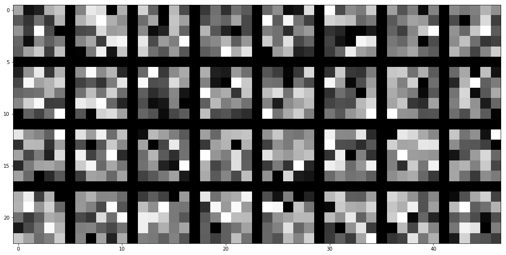
可视化

查看所有filter

kernels = sess.run(tf.reshape(tf.transpose(W_conv1, perm=[2, 3, 0 ,1]), [32, -1]))
### get tools from remote sever
import urllib.request
response = urllib.request.urlopen('http://deeplearning.net/tutorial/code/utils.py')
content = response.read().decode('utf-8')
target = open('utils1.py', 'w')
target.write(content)
target.close()

from utils1 import tile_raster_images
import matplotlib.pyplot as plt 
from PIL import Image
# %matplotlib inline
image = Image.fromarray(tile_raster_images(kernels, img_shape=(5, 5) ,tile_shape=(4, 8), tile_spacing=(1, 1)))
### Plot image
plt.rcParams['figure.figsize'] = (18.0, 18.0)
imgplot = plt.imshow(image)
imgplot.set_cmap('gray')  

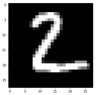
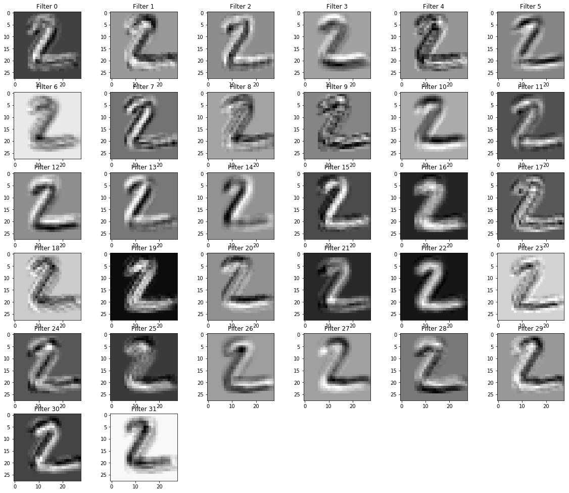
第一层卷积层的输出

import numpy as np
plt.rcParams['figure.figsize'] = (5.0, 5.0)
sampleimage = mnise.test.images[1]
plt.imshow(np.reshape(sampleimage, [28, 28]), cmap='gray')

plt.rcParams['figure.figsize'] = (5.0, 5.0)
sampleimage = mnist.test.images[1]
plt.imshow(np.reshape(sampleimage, [28, 28]), cmap='gray')
ActivatedUnits = sess.run(convolve1, feed_dict={x:np.reshape(sampleimage, [1, 784], order='F'), keep_prob:1.0})
filters = ActivatedUnits.shape[3]
plt.figure(1, figsize=(20, 20))
n_columns = 6
n_rows = np.math.ceil(filters/n_columns) + 1
for i in range(filters):
    plt.subplot(n_rows, n_columns, i+1)
    plt.title('Filters' + str(i))
    plt.imshow(ActivatedUnits[0, :, :, i], interpolation = 'nearest', cmap='gray')

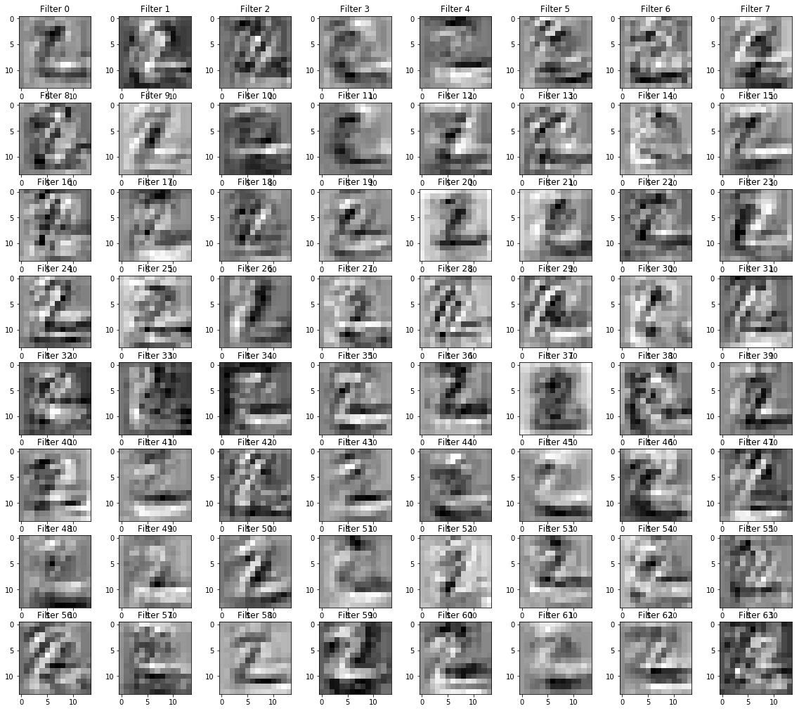
第二个卷积层的输出

ActivatedUnits = sess.run(convolve2,feed_dict={x:np.reshape(sampleimage, [1,784], order='F'), keep_prob:1.0})
filters = ActivatedUnits.shape[3]
plt.figure(1, figsize=(20,20))
n_columns = 8
n_rows = np.math.ceil(filters / n_columns) + 1
for i in range(filters):
    plt.subplot(n_rows, n_columns, i+1)
    plt.title('Filter ' + str(i))
    plt.imshow(ActivatedUnits[0, :, :, i], interpolation="nearest", cmap="gray")

结束会话

sess.close() # finish the session

References

https://en.wikipedia.org/wiki/Deep_learning
http://sebastianruder.com/optimizing-gradient-descent/index.html#batchgradientdescent
http://yann.lecun.com/exdb/mnist/
https://www.quora.com/Artificial-Neural-Networks-What-is-the-difference-between-activation-functions
https://www.tensorflow.org/versions/r0.9/tutorials/mnist/pros/index.html

---

---

本文译自 Deep Learning with TensorFlow IBM Cognitive Class ML0120EN
ML0120EN-2.2-Review-CNN-MNIST-Dataset