时间序列预测 — BiLSTM实现多变量多步光伏预测(Tensorflow)

目录

1 数据处理

1.1 导入库文件

1.2 导入数据集

1.3 缺失值分析

2 构造训练数据

3 模型训练

3.1 BiLSTM网络 

3.2 模型训练

4 模型预测

---

1 数据处理

1.1 导入库文件

import time
import datetime
import pandas as pd 
import numpy as np 
import matplotlib.pyplot as plt  
from sampen import sampen2  # sampen库用于计算样本熵
from vmdpy import VMD  # VMD分解库

import tensorflow as tf 
from sklearn.cluster import KMeans
from sklearn.metrics import r2_score, mean_squared_error, mean_absolute_error, mean_absolute_percentage_error 
from sklearn.preprocessing import MinMaxScaler
from tensorflow.keras.models import Sequential
from tensorflow.keras.layers import Dense, Activation, Dropout, LSTM, GRU
from tensorflow.keras.callbacks import ReduceLROnPlateau, EarlyStopping

# 忽略警告信息
import warnings
warnings.filterwarnings('ignore')  

1.2 导入数据集

实验数据集采用数据集8：新疆光伏风电数据集（下载链接），数据集包括组件温度(℃) 、温度(°)    气压(hPa)、湿度(%)、总辐射(W/m2)、直射辐射(W/m2)、散射辐射(W/m2)、实际发电功率(mw)特征，时间间隔15min。对数据进行可视化：

# 导入数据
data_raw = pd.read_excel("E:\\课题\\08数据集\\新疆风电光伏数据\\光伏2019.xlsx")
data_raw

from itertools import cycle
# 可视化数据
def visualize_data(data, row, col):
    cycol = cycle('bgrcmk')
    cols = list(data.columns)
    fig, axes = plt.subplots(row, col, figsize=(16, 4))
    fig.tight_layout()
    if row == 1 and col == 1:  # 处理只有1行1列的情况
        axes = [axes]  # 转换为列表，方便统一处理
    for i, ax in enumerate(axes.flat):
        if i < len(cols):
            ax.plot(data.iloc[:,i], c=next(cycol))
            ax.set_title(cols[i])
        else:
            ax.axis('off')  # 如果数据列数小于子图数量，关闭多余的子图
    plt.subplots_adjust(hspace=0.6)
    plt.show()

visualize_data(data_raw.iloc[:,1:], 2, 4)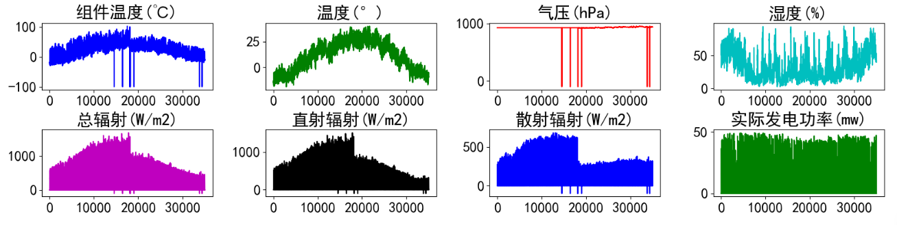

​

​单独查看部分功率数据，发现有较强的规律性。

​

​因为只是单变量预测，只选取实际发电功率(mw)数据进行实验：

1.3 缺失值分析

首先查看数据的信息，发现并没有缺失值

data_raw.info()

​

 进一步统计缺失值

data_raw.isnull().sum()

​

2 构造训练数据

构造训练数据，也是真正预测未来的关键。首先设置预测的timesteps时间步、predict_steps预测的步长（预测的步长应该比总的预测步长小），length总的预测步长，参数可以根据需要更改。

timesteps = 96*5 #构造x，为96*5个数据,表示每次用前96*5个数据作为一段
predict_steps = 96 #构造y，为96个数据，表示用后96个数据作为一段
length = 96 #预测多步，预测96个数据
feature_num = 7 #特征的数量

通过前5天的timesteps数据预测后一天的数据predict_steps个，需要对数据集进行滚动划分（也就是前timesteps行的特征和后predict_steps行的标签训练，后面预测时就可通过timesteps行特征预测未来的predict_steps个标签）。因为是多变量，特征和标签分开划分，不然后面归一化会有信息泄露的问题。

# 构造数据集，用于真正预测未来数据
# 整体的思路也就是，前面通过前timesteps个数据训练后面的predict_steps个未来数据
# 预测时取出前timesteps个数据预测未来的predict_steps个未来数据。
def create_dataset(datasetx,datasety,timesteps=36,predict_size=6):
    datax=[]#构造x
    datay=[]#构造y
    for each in range(len(datasetx)-timesteps - predict_steps):
        x = datasetx[each:each+timesteps]
        y = datasety[each+timesteps:each+timesteps+predict_steps]
        datax.append(x)
        datay.append(y)
    return datax, datay

​

数据处理前，需要对数据进行归一化，按照上面的方法划分数据，这里返回划分的数据和归一化模型，函数的定义如下：

# 数据归一化操作
def data_scaler(datax,datay):
    # 数据归一化操作
    scaler1 = MinMaxScaler(feature_range=(0,1))
    scaler2 = MinMaxScaler(feature_range=(0,1))
    datax = scaler1.fit_transform(datax)
    datay = scaler2.fit_transform(datay)
    # 用前面的数据进行训练，留最后的数据进行预测
    trainx, trainy = create_dataset(datax[:-timesteps-predict_steps,:],datay[:-timesteps-predict_steps,0],timesteps, predict_steps)
    trainx = np.array(trainx)
    trainy = np.array(trainy)
    
    return trainx, trainy, scaler1, scaler2

然后对数据按照上面的函数进行划分和归一化。通过前5天的96*5数据预测后一天的数据96个，需要对数据集进行滚动划分（也就是前96*5行的特征和后96行的标签训练，后面预测时就可通过96*5行特征预测未来的96个标签）

datax = df_vmd[:,:-1]
datay = df_vmd[:,-1].reshape(df_vmd.shape[0],1)
trainx, trainy, scaler1, scaler2 = data_scaler(datax, datay)

​

3 模型训练

3.1 BiLSTM网络 

长短期记忆神经网络（Long Short-Term Memory， LSTM） 是一种时间循环神经网络，是为
了解决一般的RNN存在的长期依赖问题而专门设计出来的，所有的RNN都具有一种重复神经
网络模块的链式形式。在标准RNN中，这个重复的结构模块只有一个非常简单的结构，例如一
个tanh层。 LSTM神经网络采用门控机制替换了循环神经网络简单的隐含层神经元， 可以解决长
期依赖的问题，在处理时序问题上表现出色。

LSTM 神经网络

传统的 LSTM 网络只能根据历史状态向前编码，无法考虑反向序列的影响。而电力负荷数
据变化与时间发展密切相关，未来数据通常与过去数据相似， 为了更全面、准确地预测，需要
考虑反向序列的影响。 双向长短期记忆神经网络（Bi-directional Long Short-Term Memory，
BiLSTM） 引入了双向计算的思想，它可以实现基于原始的 LSTM 网络同时进行正向和反向计
算， 可以同时提取前向和后向信息，更好地挖掘负荷数据的时序特征，进一步提高预测模型精度。

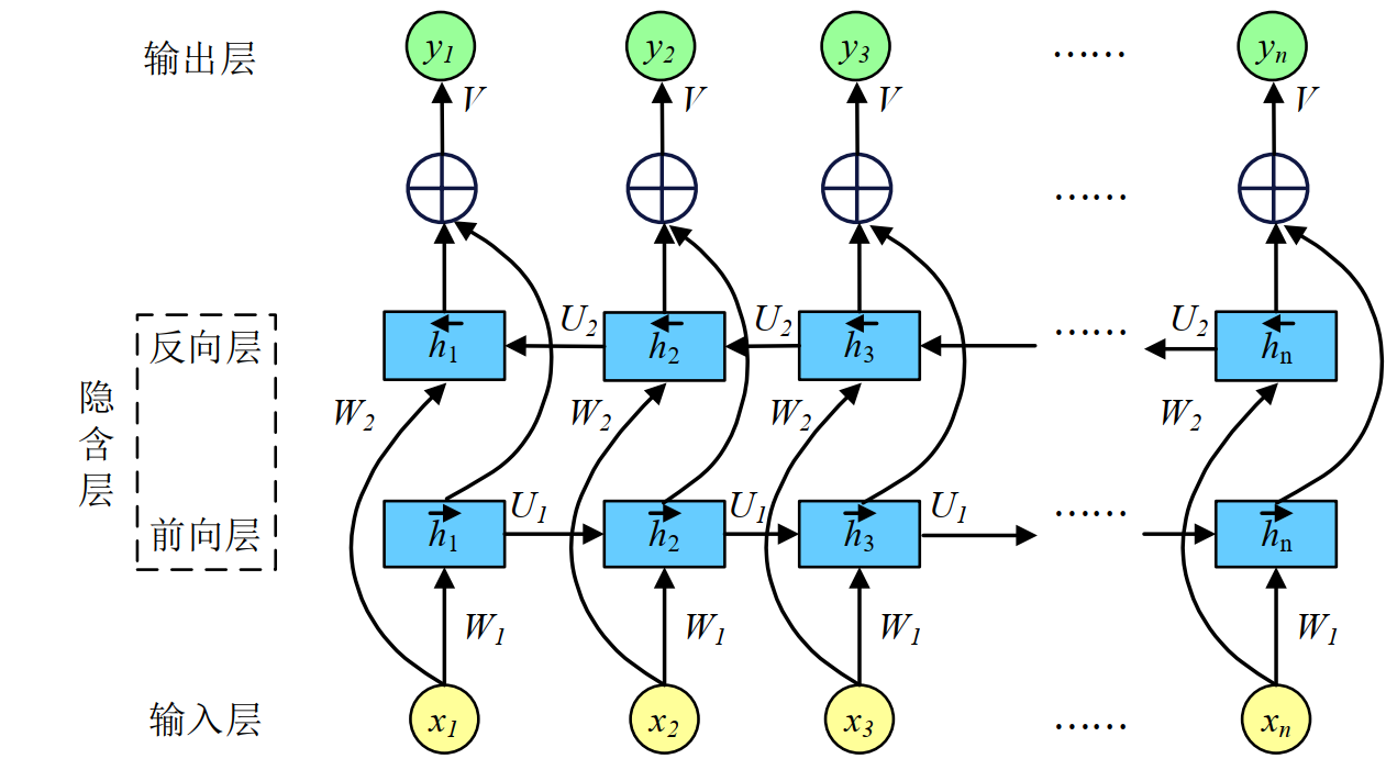
BiLSTM 神经网络

可以通过Bidirectional()来构建一个BiLSTM模型并进行训练的过程，实现主体代码如下：

    model.add(Bidirectional(LSTM(units=50, return_sequences=True), input_shape=(timesteps, feature_num)))
    model.add(Bidirectional(LSTM(units=100, return_sequences=True), input_shape=(timesteps, feature_num)))
    model.add(Bidirectional(LSTM(units=150)))

•  units=50：表示LSTM层中有50个神经元
• return_sequences=True：表示该层返回整个序列而不仅仅是输出序列的最后一个
• input_shape=(timesteps, feature_num)：表示输入数据的形状为(timesteps, feature_num)，这里timesteps和feature_num是预先定义好的输入数据的时间步数和特征数。

第一行代码向模型中再次添加了一个双向的LSTM层，使用了units=50个神经元。

第二行代码向模型中再次添加了一个双向的LSTM层，与上一行类似，但这次使用了units=100个神经元。

第三行代码向模型中添加了另一个双向的LSTM层，这次没有设置return_sequences=True，表示该层不返回整个序列，而是只返回输出序列的最后一个值。
 

3.2 模型训练

首先搭建模型的常规操作，然后使用训练数据trainx和trainy进行训练，进行50个epochs的训练，每个batch包含64个样本。此时input_shape划分数据集时每个x的形状。（建议使用GPU进行训练，因为本人电脑性能有限，建议增加epochs值；也可以依次增加LSTM网络中units）

# # 创建BiLSTM模型
def BiLSTM_model_train(trainx, trainy):
    # 调用GPU加速
    gpus = tf.config.experimental.list_physical_devices(device_type='GPU')
    for gpu in gpus:
        tf.config.experimental.set_memory_growth(gpu, True)
              
    # BiLSTM网络构建 
    start_time = datetime.datetime.now()
    model = Sequential()
    model.add(Bidirectional(LSTM(units=50, return_sequences=True), input_shape=(timesteps, feature_num)))
    model.add(Bidirectional(LSTM(units=100, return_sequences=True), input_shape=(timesteps, feature_num)))
    model.add(Bidirectional(LSTM(units=150)))
    model.add(Dropout(0.1))
    model.add(Dense(predict_steps))
    model.compile(loss='mse', optimizer='adam')
    # 模型训练
    model.fit(trainx, trainy, epochs=50, batch_size=64)
    end_time = datetime.datetime.now()
    running_time = end_time - start_time
    # 保存模型
    model.save('BiLSTM_model.h5')
    
    # 返回构建好的模型
    return model

model = BiLSTM_model_train(trainx, trainy)

4 模型预测

首先加载训练好后的模型

# 加载模型
from tensorflow.keras.models import load_model
model = load_model('BiLSTM_model.h5')

准备好需要预测的数据，训练时保留了6天的数据，将前5天的数据作为输入预测，将预测的结果和最后一天的真实值进行比较。

y_true = datay[-timesteps-predict_steps:-timesteps]
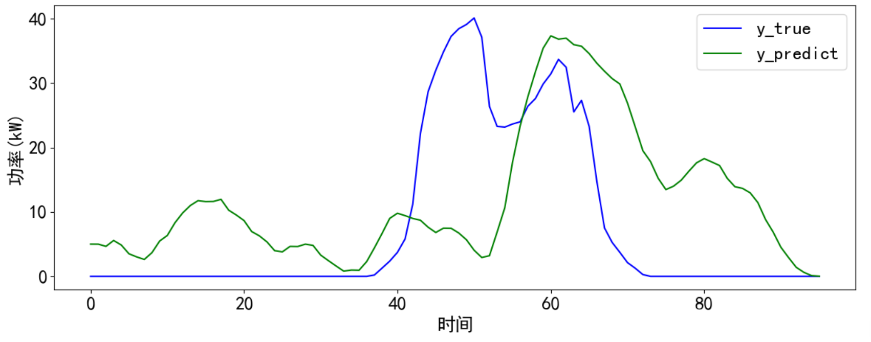
x_pred = datax[-timesteps:]

预测并计算误差，并进行可视化，将这些步骤封装为函数。

# 预测并计算误差和可视化
def predict_and_plot(x, y_true, model, scaler, timesteps):
    # 变换输入x格式，适应LSTM模型
    predict_x = np.reshape(x, (1, timesteps, feature_num))  
    # 预测
    predict_y = model.predict(predict_x)
    predict_y = scaler.inverse_transform(predict_y)
    y_predict = []
    y_predict.extend(predict_y[0])
    
    # 计算误差
    r2 = r2_score(y_true, y_predict)
    rmse = mean_squared_error(y_true, y_predict, squared=False)
    mae = mean_absolute_error(y_true, y_predict)
    mape = mean_absolute_percentage_error(y_true, y_predict)
    print("r2: %.2f\nrmse: %.2f\nmae: %.2f\nmape: %.2f" % (r2, rmse, mae, mape))
    
    # 预测结果可视化
    cycol = cycle('bgrcmk')
    plt.figure(dpi=100, figsize=(14, 5))
    plt.plot(y_true, c=next(cycol), markevery=5)
    plt.plot(y_predict, c=next(cycol), markevery=5)
    plt.legend(['y_true', 'y_predict'])
    plt.xlabel('时间')
    plt.ylabel('功率(kW)')
    plt.show()
    
    return y_predict
    

y_predict_nowork = predict_and_plot(x_pred, y_true, model, scaler2, timesteps)

最后得到可视化结果，发下可视化结果并不是太好，可以通过调参和数据处理进一步提升模型预测效果。

​