OpenCV 中的图像处理 002_图像的几何变换

本文主要内容来自于 OpenCV-Python 教程的 OpenCV 中的图像处理部分，这个部分的主要内容如下：

改变色彩空间

学习在不同色彩空间之间改变图像。另外学习跟踪视频中的彩色对象。
图像的几何变换

学习对图像应用不同的几何变换，比如旋转、平移等。
图像阈值

学习使用全局阈值、自适应阈值、Otsu 的二值化等将图像转换为二值图像。
平滑图像

学习模糊图像，使用自定义内核过滤图像等。
形态变换

了解形态学变换，如侵蚀、膨胀、开放、闭合等。
图像渐变

学习寻找图像渐变、边缘等。
Canny 边缘检测

学习通过 Canny 边缘检测寻找边缘。
图像金字塔

学习关于图像金字塔的内容，以及如何使用它们进行图像混合。
OpenCV 中的轮廓

所有关于 OpenCV 中的轮廓的内容。
OpenCV 中的直方图

所有关于 OpenCV 中的直方图的内容。
OpenCV 中的图像变换

在 OpenCV 中遇到不同的图像变换，如傅里叶变换、余弦变换等。
模板匹配

学习使用模板匹配在图像中搜索对象。
霍夫线变换

学习在一幅图像中探测线。
霍夫圆变换

学习在一幅图像中探测圆。
使用分水岭算法的图像分割

学习使用分水岭分割算法分割图像。
使用 GrabCut 算法的交互式前景提取

学习使用 GrabCut 算法提取前景

目标

学习对图像应用不同的几何变换，比如平移，旋转和仿射变换等等。
我们将看到这些函数：cv.getPerspectiveTransform。

变换

OpenCV 提供了两个变换函数，cv.warpAffine 和 cv.warpPerspective，通过它们我们可以执行所有种类的变换。cv.warpAffine 接收一个 2x3 的变换矩阵，而 cv.warpPerspective 则接收一个 3x3 的变换矩阵作为参数。

放缩

放缩只是改变图像的大小。OpenCV 有一个函数 cv.resize() 用于完成这个操作。图像的大小可以手动指定，或者可以指定放缩因子。放缩时可以使用不同的插值方法。用于缩小的首选插值方法是 cv.INTER_AREA，用于放大的是 cv.INTER_CUBIC (slow) & cv.INTER_LINEAR。默认情况下，cv.INTER_LINEAR 插值方法用于所有的调整大小。我们可以通过如下的方法改变一幅输入图像的大小：

def scaling():
    cv.samples.addSamplesDataSearchPath("/media/data/my_multimedia/opencv-4.x/samples/data")
    img = cv.imread(cv.samples.findFile('messi5.jpg'))
    res = cv.resize(img, None, fx=2, fy=2, interpolation=cv.INTER_CUBIC)
    cv.imshow('frame', res)

    # OR
    height, width = img.shape[:2]
    res = cv.resize(img, (2 * width, 2 * height), interpolation=cv.INTER_CUBIC)
    cv.waitKey()

    cv.destroyAllWindows()

放缩操作对许多以多幅图像为参数的操作比较有意义。当某个操作的输入为多幅图像，且对输入的图像的大小有一定的限制，而实际的输入图像又难以满足这种限制时，放缩可以帮我们改变部分图像的大小，以满足目标操作的输入要求。比如多幅图像的相加操作，图像的水平拼接和竖直拼接等。

平移

平移是移动一个物体的位置。如果知道了 (x,y) 方向的偏移，并使其为 ( $t_x$ , $t_y$ )，则我们可以创建如下的转换矩阵：
$\begin{bmatrix} 1&0&t_x \\ 0&1&t_x \end{bmatrix}$

$dst(x,y) = src(M_{11} ∗ x+M_{12}∗ y+M_{13}, M_{21}∗ x+M_{22}∗ y+M_{23}) \\ = src(1∗x+0∗y+t_x, 0∗x+1∗y+t_y)$

我们可以把它放入 np.float32 类型的 Numpy 数组并将其传递给 cv.warpAffine() 函数。可以参考下面移动 (100,50) 的例子：

def translation():
    cv.samples.addSamplesDataSearchPath("/media/data/my_multimedia/opencv-4.x/samples/data")
    img = cv.imread(cv.samples.findFile('messi5.jpg'))

    rows, cols, _ = img.shape
    M = np.float32([[1, 0, 100], [0, 1, 50]])
    dst = cv.warpAffine(img, M, (cols, rows))
    
    dst = cv.hconcat([img, dst])

    cv.imshow('frame', dst)
    cv.waitKey()

    cv.destroyAllWindows()

cv.warpAffine() 函数的第三个参数是输出图像的大小，它的形式应该是 (width, height)。记得 width = 列数，而 height = 行数。

看到的结果应该像下面这样：

Translation

旋转

将一幅图像旋转角度 θ，可以通过如下的转换矩阵实现：
$\begin{bmatrix} cosθ&−sinθ \\ sinθ&cosθ \end{bmatrix}$

但是 OpenCV 提供了带有可调节旋转中心的放缩旋转，因此我们可以在任何喜欢的位置旋转。修改后的变换矩阵由下式给出

$\begin{bmatrix} α&β&(1−α)⋅center.x−β⋅center.y \\ −β&α&β⋅center.x+(1−α)⋅center.y \end{bmatrix}$

其中：
$\\ β=scale⋅sinθ$

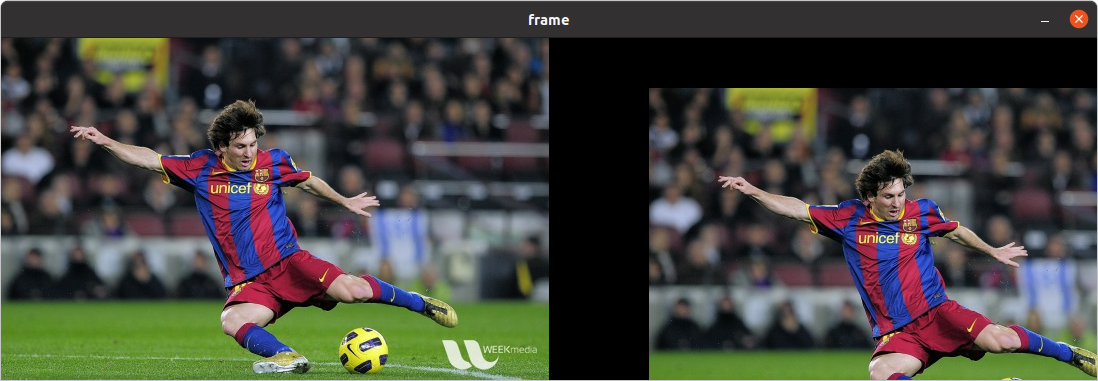
为了获得这个旋转矩阵，OpenCV 提供了一个函数，cv.getRotationMatrix2D。检查如下的例子，它将图像相对于中心旋转 120 度且放大到 1.2 倍。

def rotation():
    cv.samples.addSamplesDataSearchPath("/media/data/my_multimedia/opencv-4.x/samples/data")
    img = cv.imread(cv.samples.findFile('messi5.jpg'))

    rows, cols, _ = img.shape

    # cols-1 and rows-1 are the coordinate limits.
    M = cv.getRotationMatrix2D(((cols - 1) / 2.0, (rows - 1) / 2.0), 120, 1.2)
    dst = cv.warpAffine(img, M, (cols, rows))

    dst = cv.hconcat([img, dst])
    cv.imshow('frame', dst)
    cv.waitKey()

    cv.destroyAllWindows()

来看下结果：

Rotation

放射变换

在仿射变换中，原始图像中所有的平行线在输出的图像中依然是平行的。为了找到变换矩阵，我们需要输入图像中的三个点，以及它们在输出图像中对应的位置。cv.getAffineTransform 将创建一个 2x3 的矩阵，它将被传给 cv.warpAffine。

检查下面的例子，我们也将看到选中的点（它们用绿色标记）：

def affine_transformation():
    img = np.zeros((512, 512, 3), np.uint8)
    cv.rectangle(img, (0, 0), (512, 512), (255, 255, 255), -1)

    cv.line(img, (0, 50), (512, 50), (0, 0, 0), 3)
    cv.line(img, (0, 150), (512, 150), (0, 0, 0), 3)
    cv.line(img, (0, 300), (512, 300), (0, 0, 0), 3)
    cv.line(img, (0, 450), (512, 450), (0, 0, 0), 3)

    cv.line(img, (100, 0), (100, 512), (0, 0, 0), 3)
    cv.line(img, (256, 0), (256, 512), (0, 0, 0), 3)
    cv.line(img, (412, 0), (412, 512), (0, 0, 0), 3)

    cv.rectangle(img, (60, 170), (430, 400), (0, 0, 0), 3)

    # img, center, radius, color, thickness=None
    cv.circle(img, (60, 50), 8, (0, 255, 0), -1)
    cv.circle(img, (280, 50), 8, (0, 255, 0), -1)
    cv.circle(img, (60, 270), 8, (0, 255, 0), -1)

    rows, cols, ch = img.shape

    pts1 = np.float32([[50, 50], [200, 50], [50, 200]])
    pts2 = np.float32([[10, 100], [200, 50], [100, 250]])

    M = cv.getAffineTransform(pts1, pts2)

    dst = cv.warpAffine(img, M, (cols, rows))

    plt.subplot(121), plt.imshow(img), plt.title('Input')
    plt.subplot(122), plt.imshow(dst), plt.title('Output')
    plt.show()


if __name__ == "__main__":
    affine_transformation()

可以看到下面的结果：

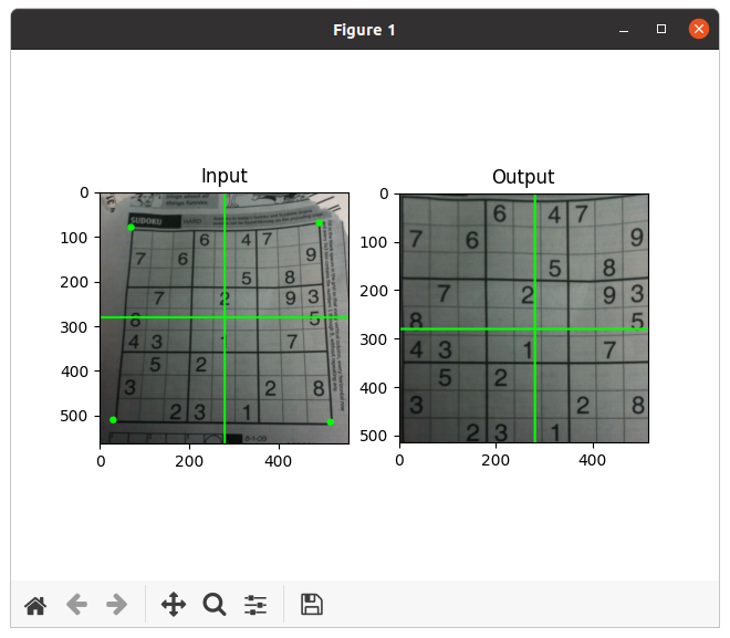
透视变换

对于透视变换，我们需要一个 3x3 的变换矩阵。即使在转换之后，直线也将保持笔直。要找到这个变换矩阵，我们需要输入图像上的 4 个点和输出图像上的对应点。这 4 个点中，有 3 个不应该共线。然后可以通过函数 cv.getPerspectiveTransform 找到变换矩阵。然后用这个 3x3 变换矩阵应用 cv.warpPerspective。

可以看下如下的代码：

def perspective_transformation():
    cv.samples.addSamplesDataSearchPath("/media/data/my_multimedia/opencv-4.x/samples/data")
    img = cv.imread(cv.samples.findFile('sudoku.png'))
    rows, cols, ch = img.shape

    pts1 = np.float32([[70, 80], [490, 70], [30, 510], [515, 515]])
    pts2 = np.float32([[0, 0], [515, 0], [0, 515], [515, 515]])
    M = cv.getPerspectiveTransform(pts1, pts2)
    dst = cv.warpPerspective(img, M, (515, 515))

    cv.line(img, (0, int(rows / 2)), (cols, int(rows / 2)), (0, 255, 0), 3)
    cv.line(img, (int(cols / 2), 0), (int(cols / 2), rows), (0, 255, 0), 3)

    cv.circle(img, (70, 80), 8, (0, 255, 0), -1)
    cv.circle(img, (490, 70), 8, (0, 255, 0), -1)
    cv.circle(img, (30, 510), 8, (0, 255, 0), -1)
    cv.circle(img, (515, 515), 8, (0, 255, 0), -1)

    plt.subplot(121), plt.imshow(img), plt.title('Input')

    cv.line(dst, (0, int(rows / 2)), (cols, int(rows / 2)), (0, 255, 0), 3)
    cv.line(dst, (int(cols / 2), 0), (int(cols / 2), rows), (0, 255, 0), 3)
    plt.subplot(122), plt.imshow(dst), plt.title('Output')
    plt.show()


if __name__ == "__main__":
    perspective_transformation()

最终的结果如下图：